Chapter 2: The Language of Probability: Sets, Sample Spaces, and Events

Welcome to Chapter 2! In the previous chapter, we introduced the ‘why’ of probability and set up our Python environment. Now, we dive into the fundamental vocabulary and concepts that form the bedrock of probability theory. Understanding these core ideas – sample spaces, events, and the rules governing them – is crucial before we can tackle more complex problems and distributions. We’ll use set theory as our language and Python to make these abstract concepts tangible.

Learning Objectives¶

• Understand and define experiments, outcomes, and sample spaces.

• Distinguish between discrete and continuous sample spaces.

• Define events as subsets of the sample space.

• Review basic set operations (union, intersection, complement) and their relevance to probability.

• Grasp the fundamental Axioms of Probability.

• Apply basic probability rules like the Complement and Addition rules.

• Use Python sets and lists to represent sample spaces and events.

• Calculate empirical probabilities through simulation.

Experiments, Outcomes, Sample Spaces¶

In probability, an experiment is any procedure or process that can be repeated infinitely (in theory) and has a well-defined set of possible results. Think of flipping a coin, rolling a die, measuring a patient’s temperature, or recording the time it takes for a website to load.

Each possible result of an experiment is called an outcome.

• For flipping a coin, the outcomes are Heads (H) or Tails (T).

• For rolling a standard six-sided die, the outcomes are the integers 1, 2, 3, 4, 5, 6.

• For measuring temperature, an outcome could be 37.2°C.

• For website load time, an outcome could be 1.34 seconds.

The sample space, often denoted by $S$ or $\Omega$ (Omega), is the set of all possible outcomes of an experiment.

Discrete vs. Continuous Sample Spaces¶

Sample spaces can be categorized based on the nature of their outcomes:

1. Discrete Sample Space: Contains a finite or countably infinite number of outcomes. The outcomes can be listed.

   • Example (Finite): Rolling a standard six-sided die. The sample space is $S = \{1, 2, 3, 4, 5, 6\}$.

   • Example (Countably Infinite): Flipping a coin until the first Head appears. The sample space is $S = \{H, TH, TTH, TTTH, ...\}$. Although infinite, we can map each outcome to a positive integer (1st flip, 2nd flip, 3rd flip, etc.).

2. Continuous Sample Space: Contains an infinite number of outcomes that form a continuum. The outcomes cannot be listed individually because there are infinitely many possibilities between any two given outcomes.

   • Example: Measuring the exact height of a randomly selected adult. The sample space might be all real numbers between 0.5 meters and 3.0 meters, $S = \{h \in \mathbb{R} \mid 0.5 \le h \le 3.0\}$.

   • Example: Recording the time until a component fails. $S = \{t \in \mathbb{R} \mid t \ge 0\}$.

Python Representation (Discrete): We can easily represent finite discrete sample spaces using Python sets or lists. Sets are often conceptually closer as they inherently handle uniqueness and order doesn’t matter.

# Sample space for rolling a single six-sided die
sample_space_die = {1, 2, 3, 4, 5, 6}

# Sample space for flipping a coin
sample_space_coin = {'Heads', 'Tails'}

print(f"Sample space (Die): {sample_space_die}")
print(f"Sample space (Coin): {sample_space_coin}")

Sample space (Die): {1, 2, 3, 4, 5, 6}
Sample space (Coin): {'Heads', 'Tails'}

Events as Subsets¶

An event is any subset of the sample space. It represents a specific outcome or a collection of outcomes of interest. Events are usually denoted by capital letters (A, B, E, etc.).

• Experiment: Rolling a die ($S = \{1, 2, 3, 4, 5, 6\}$)

  • Event A: Rolling an even number. $A = \{2, 4, 6\}$. Note that $A \subseteq S$.

  • Event B: Rolling a number greater than 4. $B = \{5, 6\}$. Note that $B \subseteq S$.

  • Event C: Rolling a 3. $C = \{3\}$. Simple event (contains only one outcome).

  • Event D: Rolling a number less than 10. $D = \{1, 2, 3, 4, 5, 6\} = S$. This is the certain event.

  • Event E: Rolling a 7. $E = \{\}$ or $\emptyset$. This is the impossible event (the empty set).

Python Representation: Events, being subsets, can also be represented using Python sets.

# Continuing the die roll example
S = {1, 2, 3, 4, 5, 6}

# Event A: Rolling an even number
A = {2, 4, 6}

# Event B: Rolling a number greater than 4
B = {5, 6}

# Check if they are subsets of S
print(f"Is A a subset of S? {A.issubset(S)}")
print(f"Is B a subset of S? {B.issubset(S)}")
print(f"Event A: {A}")
print(f"Event B: {B}")

Is A a subset of S? True
Is B a subset of S? True
Event A: {2, 4, 6}
Event B: {5, 6}

Set Theory Refresher¶

Since events are sets, the language and operations of set theory are fundamental to probability. Let A and B be two events in a sample space S.

1. Union ($A \cup B$): The set of outcomes that are in A, or in B, or in both. Corresponds to the logical ‘OR’.

   • Example: For the die roll, $A \cup B$ = “Rolling an even number OR a number greater than 4” = $\{2, 4, 5, 6\}$.

2. Intersection ($A \cap B$): The set of outcomes that are in both A and B. Corresponds to the logical ‘AND’.

   • Example: For the die roll, $A \cap B$ = “Rolling an even number AND a number greater than 4” = $\{6\}$.

3. Complement ($A'$ or $A^c$): The set of outcomes in the sample space S that are not in A. Corresponds to the logical ‘NOT’.

   • Example: For the die roll, $A'$ = “NOT rolling an even number” = “Rolling an odd number” = $\{1, 3, 5\}$.

Disjoint Events: Two events A and B are disjoint or mutually exclusive if they have no outcomes in common, i.e., their intersection is the empty set ($A \cap B = \emptyset$).

• Example: The event “Rolling an even number” (A={2,4,6}) and the event “Rolling an odd number” (A’={1,3,5}) are disjoint. The event “Rolling a 1” ({1}) and “Rolling a 6” ({6}) are disjoint.

Venn Diagrams: These are useful visual aids. The sample space S is represented by a rectangle, and events are represented by circles or shapes within it. Overlapping areas show intersections, and the area outside a circle represents its complement.

(We won’t draw Venn diagrams directly in code here, but libraries like matplotlib_venn can be used for this. Conceptually, imagine S as a box containing numbers 1-6. Circle A encloses 2, 4, 6. Circle B encloses 5, 6. The overlap contains only 6. The area outside A contains 1, 3, 5.)

Python Set Operations:

S = {1, 2, 3, 4, 5, 6}
A = {2, 4, 6}  # Even numbers
B = {5, 6}     # Numbers > 4
C = {1, 3, 5}  # Odd numbers (A's complement)

# Union (A or B)
union_AB = A.union(B)
print(f"A union B: {union_AB}") # Corresponds to {2, 4, 5, 6}

# Intersection (A and B)
intersection_AB = A.intersection(B)
print(f"A intersection B: {intersection_AB}") # Corresponds to {6}

# Complement of A (relative to S)
complement_A = S.difference(A)
print(f"Complement of A: {complement_A}") # Corresponds to {1, 3, 5}
print(f"Is complement of A equal to C? {complement_A == C}")

# Check for disjoint events (A and C)
intersection_AC = A.intersection(C)
print(f"A intersection C: {intersection_AC}") # Corresponds to {}
print(f"Are A and C disjoint? {intersection_AC == set()}") # Empty set means disjoint

A union B: {2, 4, 5, 6}

A intersection B: {6}
Complement of A: {1, 3, 5}
Is complement of A equal to C? True
A intersection C: set()
Are A and C disjoint? True

Axioms of Probability¶

The entire structure of probability theory is built upon three fundamental axioms, proposed by Andrey Kolmogorov. Let S be a sample space, and P(A) denote the probability of an event A.

1. Non-negativity: For any event A, the probability of A is greater than or equal to zero.

   $$P(A) \ge 0$$

   (1)

   Probabilities cannot be negative.

2. Normalization: The probability of the entire sample space S is equal to 1.

   $$P(S) = 1$$

   (2)

   This means that some outcome within the realm of possibility must occur. The maximum possible probability is 1.

3. Additivity for Disjoint Events: If $A_1, A_2, A_3, ...$ is a sequence of mutually exclusive (disjoint) events (i.e., $A_i \cap A_j = \emptyset$ for all $i \ne j$), then the probability of their union is the sum of their individual probabilities:

   $$P(A_1 \cup A_2 \cup A_3 \cup ...) = P(A_1) + P(A_2) + P(A_3) + ...$$

   (3)

   For a finite number of disjoint events, say A and B, this simplifies to: If $A \cap B = \emptyset$, then $P(A \cup B) = P(A) + P(B)$.

Examples based on the axioms:

Consider rolling a fair six-sided die with $S = \{1, 2, 3, 4, 5, 6\}$. Assuming fairness, each outcome has probability 1/6.

Example 1 - Non-negativity (Axiom 1):

Each individual outcome has non-negative probability:

Example 2 - Normalization (Axiom 2):

The event “Roll < 7” equals the entire sample space: $D = \{1, 2, 3, 4, 5, 6\} = S$.

Since the individual outcomes are disjoint, we can apply Axiom 3:

Example 3 - Impossible events:

The event “Roll > 6” is impossible: $E = \emptyset$.

To find $P(\emptyset)$, note that $S \cup \emptyset = S$ and these sets are disjoint. By Axiom 3:

Since $P(S) = 1$ (Axiom 2):

This shows that the probability of any impossible event is 0.

Basic Probability Rules¶

Several useful rules can be derived directly from the axioms:

1. Probability Range: For any event A:

   $$0 \le P(A) \le 1$$

   (11)

   (Follows from Axioms 1 & 2 and $A \subseteq S$).

2. Complement Rule: The probability that event A does not occur is 1 minus the probability that it does occur.

   $$P(A') = 1 - P(A)$$

   (12)

   • Derivation: A and A’ are disjoint ($A \cap A' = \emptyset$) and their union is the entire sample space ($A \cup A' = S$). By Axiom 3, $P(A \cup A') = P(A) + P(A')$. By Axiom 2, $P(S) = 1$. Therefore, $P(A) + P(A') = 1$, which rearranges to the rule.

   • Example: What is the probability of not rolling a 6? Let $A = \{6\}$, so $P(A) = 1/6$. $A'$ = “not rolling a 6” = $\{1, 2, 3, 4, 5\}$. $P(A') = 1 - P(A) = 1 - 1/6 = 5/6$.

3. Addition Rule (General): For any two events A and B (not necessarily disjoint), the probability that A or B (or both) occurs is:

   $$P(A \cup B) = P(A) + P(B) - P(A \cap B)$$

   (13)

   • Intuition: If we simply add P(A) and P(B), we have double-counted the probability of the outcomes that are in both A and B (the intersection). So, we subtract $P(A \cap B)$ to correct for this. If A and B are disjoint, $A \cap B = \emptyset$ and $P(A \cap B) = 0$, which reduces this rule to Axiom 3 for two events.

   • Example: What is the probability of rolling an even number (A={2,4,6}) or a number greater than 4 (B={5,6})? $P(A) = 3/6 = 1/2$ $P(B) = 2/6 = 1/3$ The intersection is $A \cap B = \{6\}$, so $P(A \cap B) = 1/6$. Using the Addition Rule: $P(A \cup B) = P(A) + P(B) - P(A \cap B) = 3/6 + 2/6 - 1/6 = 4/6 = 2/3$. Let’s check the outcomes in $A \cup B = \{2, 4, 5, 6\}$. There are 4 outcomes, each with probability 1/6. So the total probability is indeed $4 \times (1/6) = 4/6 = 2/3$. It works!

Hands-on Python Practice¶

Let’s use Python to solidify these concepts through simulation. We often don’t know the theoretical probabilities beforehand, or the situation is too complex to calculate. Simulation allows us to estimate probabilities by running the experiment many times and observing the outcomes. This estimated probability is called the empirical probability.

Empirical Probability:

The Law of Large Numbers (which we’ll study later) tells us that as the number of trials increases, the empirical probability converges to the true theoretical probability.

Setup: We’ll need NumPy for efficient random number generation.

import numpy as np
import matplotlib.pyplot as plt

# Configure plots for better readability
plt.style.use('seaborn-v0_8-whitegrid')

With our libraries imported, we can now work through several examples demonstrating how Python helps us understand probability concepts.

1. Representing Sample Spaces and Events¶

We’ve already seen how to use Python sets. Let’s reiterate for a coin flip.

# Sample Space
S_coin = {'H', 'T'} # Using H for Heads, T for Tails

# Events
E_heads = {'H'}
E_tails = {'T'}

print(f"Sample Space (Coin): {S_coin}")
print(f"Event (Heads): {E_heads}")
print(f"Is Heads an event in S_coin? {E_heads.issubset(S_coin)}")

Sample Space (Coin): {'T', 'H'}
Event (Heads): {'H'}
Is Heads an event in S_coin? True

2. Simulating Simple Experiments¶

Let’s simulate rolling a fair six-sided die many times.

import numpy as np

# Simulate 1000 dice rolls
num_rolls = 1000
rolls = np.random.randint(1, 7, size=num_rolls) # Generate random integers between 1 (inclusive) and 7 (exclusive)

# Display the first 20 rolls
print(f"First 20 rolls: {rolls[:20]}")
print(f"Total rolls simulated: {len(rolls)}")

First 20 rolls: [2 2 2 6 4 4 4 6 5 5 1 6 3 3 1 3 2 6 4 6]
Total rolls simulated: 1000

3. Calculating Empirical Probabilities¶

Example: What is the empirical probability of rolling a number greater than 4?

Theoretical answer: Event $B = \{5, 6\}$. $P(B) = 2/6 = 1/3 \approx 0.333$.

# Define the event B: rolling > 4
# We can count how many rolls satisfy this condition
outcomes_greater_than_4 = rolls[rolls > 4]
num_success = len(outcomes_greater_than_4)

# Calculate empirical probability
empirical_prob_B = num_success / num_rolls

print(f"Number of rolls > 4: {num_success}")
print(f"Total rolls: {num_rolls}")
print(f"Empirical P(Roll > 4): {empirical_prob_B:.4f}")
print(f"Theoretical P(Roll > 4): {1/3:.4f}")

Number of rolls > 4: 324
Total rolls: 1000
Empirical P(Roll > 4): 0.3240
Theoretical P(Roll > 4): 0.3333

Note: The rolls variable used here comes from the dice roll simulation above. Try running the simulation and this calculation multiple times—you’ll notice the empirical probability fluctuates slightly but remains close to the theoretical value of 1/3, especially with a large num_rolls.

Example: What is the empirical probability of rolling an even number?

Theoretical answer: Event $A = \{2, 4, 6\}$. $P(A) = 3/6 = 0.5$.

# Event A: rolling an even number
# An outcome is even if outcome % 2 == 0
outcomes_even = rolls[rolls % 2 == 0]
num_even = len(outcomes_even)

# Calculate empirical probability
empirical_prob_A = num_even / num_rolls

print(f"Number of even rolls: {num_even}")
print(f"Total rolls: {num_rolls}")
print(f"Empirical P(Roll is Even): {empirical_prob_A:.4f}")
print(f"Theoretical P(Roll is Even): {0.5:.4f}")

Number of even rolls: 473
Total rolls: 1000
Empirical P(Roll is Even): 0.4730
Theoretical P(Roll is Even): 0.5000

4. Visualizing Events and Outcomes¶

We can use histograms to visualize the distribution of outcomes from our simulation.

Python Implementation

import matplotlib.pyplot as plt

# Plotting the frequency of each outcome
plt.figure(figsize=(8, 5))

# Count occurrences of each die face
faces = [1, 2, 3, 4, 5, 6]
counts = [np.sum(rolls == face) for face in faces]

# Create bar plot
plt.bar(faces, counts, color='skyblue', edgecolor='black', alpha=0.7)
plt.title(f'Frequency of Outcomes for {num_rolls} Die Rolls')
plt.xlabel('Die Face')
plt.ylabel('Frequency Count')
plt.xticks(faces)

# Add a line for the expected frequency for a fair die
expected_frequency = num_rolls / 6
plt.axhline(expected_frequency, color='red', linestyle='--', label=f'Expected Frequency ({expected_frequency:.1f})')
plt.legend()

plt.show()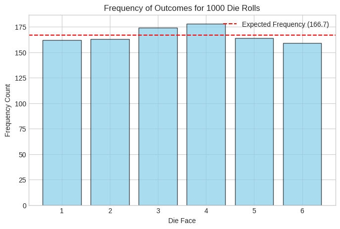

The histogram shows the counts for each outcome (1 through 6). For a fair die and a large number of rolls, we expect the bars to be roughly the same height, close to the theoretical expected frequency (total rolls / 6).

We can also visualize the outcomes that constitute a specific event. For instance, let’s highlight the rolls that were greater than 4.

# Create a boolean mask for the event
event_mask_B = rolls > 4 # True if roll > 4, False otherwise

# Simple textual visualization: show rolls and whether they met the condition
print("Roll | > 4?")
print("----|----")
for i in range(15): # Show first 15
    print(f"{rolls[i]:<4}| {event_mask_B[i]}")

# Highlight on a plot (can be more complex, here just re-emphasize the count)
print(f"\nFrom the simulation:")
print(f"- The event 'Roll > 4' (outcomes {5, 6}) occurred {num_success} times.")
print(f"- The empirical probability is {empirical_prob_B:.4f}")

Roll | > 4?
----|----
2   | False
2   | False
2   | False
6   | True
4   | False
4   | False
4   | False
6   | True
5   | True
5   | True
1   | False
6   | True
3   | False
3   | False
1   | False

From the simulation:
- The event 'Roll > 4' (outcomes (5, 6)) occurred 324 times.
- The empirical probability is 0.3240

This visualization shows which specific outcomes from our simulation satisfy the event condition (rolling > 4). It demonstrates how we can programmatically filter and analyze events from our simulated data.

Chapter Summary¶

This chapter introduced the basic language of probability theory, grounded in set theory.

• We defined experiments, outcomes, and sample spaces (discrete and continuous).

• We conceptualized events as subsets of the sample space.

• We reviewed set operations (union, intersection, complement) and how they relate to combining or modifying events.

• We established the foundational Axioms of Probability (Non-negativity, Normalization, Additivity).

• We derived essential rules like the Complement Rule and the Addition Rule.

• Crucially, we used Python to represent these concepts (using sets and numpy) and performed simulations to calculate empirical probabilities, comparing them to theoretical values.

Understanding this vocabulary and these basic rules is essential. In the next chapter, we will build upon this foundation by learning systematic ways to count the number of outcomes in sample spaces and events, which is often necessary for calculating theoretical probabilities, especially when outcomes are equally likely.

Exercises¶

1. Set Operations and Events: In a survey of 100 students:

   • 60 students study Mathematics (M)

   • 50 students study Physics (P)

   • 30 students study both Mathematics and Physics

   a) How many students study Mathematics or Physics (or both)? b) How many students study neither Mathematics nor Physics? c) How many students study exactly one of the two subjects?

   Answer

   Let $M$ be the set of students studying Mathematics, $P$ be the set of students studying Physics.

   Given:

   • $|M| = 60$

   • $|P| = 50$

   • $|M \cap P| = 30$

   • Total students = 100

   a) Students studying M or P (or both): Using the inclusion-exclusion principle:

   $$|M \cup P| = |M| + |P| - |M \cap P| = 60 + 50 - 30 = 80$$

   (15)

   Answer: 80 students

   b) Students studying neither: $|(M \cup P)^c| = 100 - |M \cup P| = 100 - 80 = 20$

   Answer: 20 students

   c) Students studying exactly one subject: Only M: $|M| - |M \cap P| = 60 - 30 = 30$ Only P: $|P| - |M \cap P| = 50 - 30 = 20$ Total: $30 + 20 = 50$

   Answer: 50 students

2. Probability Axioms: A box contains 5 red balls, 3 blue balls, and 2 green balls. You randomly select one ball.

   a) What is the probability of selecting a red ball? b) What is the probability of not selecting a red ball? c) What is the probability of selecting a red or blue ball? d) Verify that the probabilities of all possible outcomes sum to 1.

   Answer

   Sample space: $S = \{\text{Red}, \text{Blue}, \text{Green}\}$ Total balls = $5 + 3 + 2 = 10$

   a) Probability of red:

   $$P(\text{Red}) = \frac{5}{10} = \frac{1}{2} = 0.5$$

   (16)

   b) Probability of not red (Complement Rule):

   $$P(\text{Red}^c) = 1 - P(\text{Red}) = 1 - 0.5 = 0.5$$

   (17)

   Or directly: $P(\text{Blue or Green}) = \frac{3+2}{10} = \frac{5}{10} = 0.5$

   c) Probability of red or blue (Addition Rule for mutually exclusive events):

   $$P(\text{Red} \cup \text{Blue}) = P(\text{Red}) + P(\text{Blue}) = \frac{5}{10} + \frac{3}{10} = \frac{8}{10} = 0.8$$

   (18)

   d) Verification (Normalization Axiom):

   $$P(\text{Red}) + P(\text{Blue}) + P(\text{Green}) = \frac{5}{10} + \frac{3}{10} + \frac{2}{10} = \frac{10}{10} = 1 \,\checkmark$$

   (19)

3. Addition Rule: A fair six-sided die is rolled. Let $A$ be the event “roll an even number” and $B$ be the event “roll a number greater than 3”.

   a) List the outcomes in events $A$, $B$, and $A \cap B$ b) Calculate $P(A)$, $P(B)$, and $P(A \cap B)$ c) Use the Addition Rule to find $P(A \cup B)$ d) Verify your answer by directly counting favorable outcomes

   Answer

   Sample space: $S = \{1, 2, 3, 4, 5, 6\}$, each outcome has probability $\frac{1}{6}$

   a) Events:

   • $A = \{2, 4, 6\}$ (even numbers)

   • $B = \{4, 5, 6\}$ (greater than 3)

   • $A \cap B = \{4, 6\}$ (even AND greater than 3)

   b) Probabilities:

   • $P(A) = \frac{3}{6} = \frac{1}{2}$

   • $P(B) = \frac{3}{6} = \frac{1}{2}$

   • $P(A \cap B) = \frac{2}{6} = \frac{1}{3}$

   c) Using Addition Rule:

   $$P(A \cup B) = P(A) + P(B) - P(A \cap B) = \frac{1}{2} + \frac{1}{2} - \frac{1}{3} = 1 - \frac{1}{3} = \frac{2}{3}$$

   (20)

   d) Direct verification: $A \cup B = \{2, 4, 5, 6\}$, so $P(A \cup B) = \frac{4}{6} = \frac{2}{3}$ ✓

4. De Morgan’s Laws: In a deck of 52 playing cards, let:

   • $H$ = event that the card is a Heart

   • $F$ = event that the card is a face card (Jack, Queen, King)

   Find the probability that a randomly drawn card is: a) Neither a Heart nor a face card (use De Morgan’s Law: $(H \cup F)^c = H^c \cap F^c$) b) Verify your answer by calculating directly

   Answer

   In a standard deck:

   • Hearts: 13 cards, so $P(H) = \frac{13}{52} = \frac{1}{4}$

   • Face cards: $3 \times 4 = 12$ cards (J, Q, K in each suit), so $P(F) = \frac{12}{52} = \frac{3}{13}$

   • Heart face cards: 3 cards (J♥, Q♥, K♥), so $P(H \cap F) = \frac{3}{52}$

   a) Using De Morgan’s Law:

   First, find $P(H \cup F)$ using the Addition Rule:

   $$P(H \cup F) = P(H) + P(F) - P(H \cap F) = \frac{13}{52} + \frac{12}{52} - \frac{3}{52} = \frac{22}{52} = \frac{11}{26}$$

   (21)

   Then apply Complement Rule:

   $$P((H \cup F)^c) = P(H^c \cap F^c) = 1 - P(H \cup F) = 1 - \frac{11}{26} = \frac{15}{26}$$

   (22)

   b) Direct calculation: Total cards: 52 Hearts or face cards: 22 (calculated above) Neither: $52 - 22 = 30$

   $$P(H^c \cap F^c) = \frac{30}{52} = \frac{15}{26}$$

   (23)

   ✓

5. Mutually Exclusive vs. Independent: Consider rolling a fair six-sided die.

   • Let $A$ = “roll a 2”

   • Let $B$ = “roll an odd number”

   a) Are events $A$ and $B$ mutually exclusive? Explain. b) Calculate $P(A)$, $P(B)$, and $P(A \cap B)$ c) If events were independent, what would $P(A \cap B)$ equal? Compare with your answer in (b).

   Answer

   a) Mutually exclusive?

   Yes, $A$ and $B$ are mutually exclusive because:

   • $A = \{2\}$

   • $B = \{1, 3, 5\}$

   • $A \cap B = \emptyset$ (cannot roll both 2 and an odd number simultaneously)

   b) Probabilities:

   • $P(A) = \frac{1}{6}$

   • $P(B) = \frac{3}{6} = \frac{1}{2}$

   • $P(A \cap B) = 0$ (since $A \cap B = \emptyset$)

   c) If independent:

   If $A$ and $B$ were independent, then:

   $$P(A \cap B) = P(A) \times P(B) = \frac{1}{6} \times \frac{1}{2} = \frac{1}{12}$$

   (24)

   But we found $P(A \cap B) = 0 \neq \frac{1}{12}$

   Conclusion: Events $A$ and $B$ are NOT independent. Mutually exclusive events (with positive probability) can never be independent—knowing one occurred tells us the other didn’t occur.