Chapter 4: Conditional Probability

Let’s use Python to explore the concepts of conditional probability. We’ll need libraries like numpy for numerical operations and random sampling, and potentially pandas for handling data.

import numpy as np
import pandas as pd
import random

Simulating Conditional Events: Drawing Cards¶

Let’s simulate drawing two cards from a standard 52-card deck without replacement and verify the conditional probability $P(\text{2nd is King} | \text{1st is King})$. We expect this to be $3/51$.

We can also estimate the overall probability $P(\text{2nd is King})$. By symmetry or using the Law of Total Probability, this should be $4/52$.

So, both our intuition and a more formal application of probability rules confirm these results! Now, are you ready to simulate this?

# Represent the deck
ranks = ['2', '3', '4', '5', '6', '7', '8', '9', 'T', 'J', 'Q', 'K', 'A']
suits = ['H', 'D', 'C', 'S'] # Hearts, Diamonds, Clubs, Spades
deck = [rank + suit for rank in ranks for suit in suits]
kings = {'KH', 'KD', 'KC', 'KS'}

# Simulation parameters
num_simulations = 100000

# Counters
count_first_king = 0
count_second_king = 0
count_both_king = 0
count_second_king_given_first_king = 0

# Run simulations
for _ in range(num_simulations):
    # Shuffle the deck implicitly by drawing random samples
    drawn_cards = random.sample(deck, 2)
    card1 = drawn_cards[0]
    card2 = drawn_cards[1]

    # Check conditions
    is_first_king = card1 in kings
    is_second_king = card2 in kings

    if is_first_king:
        count_first_king += 1
        if is_second_king:
            count_second_king_given_first_king += 1

    if is_second_king:
        count_second_king += 1

    if is_first_king and is_second_king:
        count_both_king += 1

# Calculate probabilities from simulation
prob_first_king_sim = count_first_king / num_simulations
prob_second_king_sim = count_second_king / num_simulations
prob_both_king_sim = count_both_king / num_simulations

# Calculate conditional probability P(B|A) = P(A and B) / P(A)
# We can estimate this directly from the counts:
if count_first_king > 0:
    prob_second_given_first_sim = count_second_king_given_first_king / count_first_king
else:
    prob_second_given_first_sim = 0

# Theoretical values
prob_first_king_theory = 4/52
prob_second_king_theory = 4/52 # By symmetry
prob_both_king_theory = (4/52) * (3/51)
prob_second_given_first_theory = 3/51

# Print results
print(f"--- Theoretical Probabilities ---")
print(f"P(1st is King): {prob_first_king_theory:.6f} ({4}/{52})")
print(f"P(2nd is King): {prob_second_king_theory:.6f} ({4}/{52})")
print(f"P(Both Kings): {prob_both_king_theory:.6f}")
print(f"P(2nd is King | 1st is King): {prob_second_given_first_theory:.6f} ({3}/{51})")
print("\n")
print(f"--- Simulation Results ({num_simulations} runs) ---")
print(f"Estimated P(1st is King): {prob_first_king_sim:.6f}")
print(f"Estimated P(2nd is King): {prob_second_king_sim:.6f}")
print(f"Estimated P(Both Kings): {prob_both_king_sim:.6f}")
print(f"Estimated P(2nd is King | 1st is King): {prob_second_given_first_sim:.6f}")

--- Theoretical Probabilities ---
P(1st is King): 0.076923 (4/52)
P(2nd is King): 0.076923 (4/52)
P(Both Kings): 0.004525
P(2nd is King | 1st is King): 0.058824 (3/51)


--- Simulation Results (100000 runs) ---
Estimated P(1st is King): 0.078520
Estimated P(2nd is King): 0.078240
Estimated P(Both Kings): 0.004930
Estimated P(2nd is King | 1st is King): 0.062787

The simulation results should be very close to the theoretical values, demonstrating how simulation can approximate probabilistic calculations. The larger num_simulations, the closer the estimates will typically be.

Calculating Conditional Probabilities from Data¶

Imagine we have data about website visitors, including whether they made a purchase and whether they visited a specific product page first. We can use Pandas to calculate conditional probabilities from this data.

Sample Data¶

A DataFrame is created with data on website visitors, including whether they visited a specific product page and whether they made a purchase.

import pandas as pd

# Create sample data
data = {
    'visited_product_page': [True, False, True, True, False, False, True, True, False, True],
    'made_purchase':        [True, False, False, True, False, True, False, True, False, False]
}
df = pd.DataFrame(data)

print("Sample Visitor Data:")
display(df)
print("\n")

Sample Visitor Data:

Approach 1: Calculated Conditional Probability¶

First calculate basic probabilities:

• Basic Probabilities: The total number of visitors, visitors who visited the product page, visitors who made a purchase, and visitors who both visited the product page and made a purchase are calculated. These are used to compute the basic probabilities:

  • $P(\text{Visited Page})$

  • $P(\text{Purchased})$

  • $P(\text{Visited and Purchased})$

# Calculate basic probabilities
n_total = len(df)
n_visited_page = df['visited_product_page'].sum()
n_purchased = df['made_purchase'].sum()
n_visited_and_purchased = len(df[(df['visited_product_page'] == True) & (df['made_purchase'] == True)])

P_visited = n_visited_page / n_total
P_purchased = n_purchased / n_total
P_visited_and_purchased = n_visited_and_purchased / n_total

print(f"P(Visited Page) = {P_visited:.2f}")
print(f"P(Purchased) = {P_purchased:.2f}")
print(f"P(Visited and Purchased) = {P_visited_and_purchased:.2f}")
print("\n")

P(Visited Page) = 0.60
P(Purchased) = 0.40
P(Visited and Purchased) = 0.30

Next calculate conditional probabilities:

• Definition: This approach uses the fundamental rules of probability to derive conditional probabilities.

• Calculations:

  • $P(\text{Purchased} \mid \text{Visited Page})$: Calculated using the formula $P(A \mid B) = \frac{P(A \cap B)}{P(B)}$, where $A$ is “Purchased” and $B$ is “Visited Page”.

  • $P(\text{Visited Page} \mid \text{Purchased})$: Similarly calculated using the same probability rule.

• Advantage: This method is useful when you already have the probabilities $P(A \cap B)$ and $P(B)$ and want to use them to find the conditional probability. It’s also helpful for understanding the theoretical underpinnings of conditional probability.

# Calculate Conditional Probability: P(Purchase | Visited Page)
if P_visited > 0:
    P_purchased_given_visited = P_visited_and_purchased / P_visited
    print(f"Calculated P(Purchased | Visited Page) = {P_purchased_given_visited:.2f}")
else:
    print("Cannot calculate P(Purchased | Visited Page) as P(Visited Page) is 0.")

# Calculate Conditional Probability: P(Visited Page | Purchased)
if P_purchased > 0:
    P_visited_given_purchased = P_visited_and_purchased / P_purchased
    print(f"Calculated P(Visited Page | Purchased) = {P_visited_given_purchased:.2f}")
else:
    print("Cannot calculate P(Visited Page | Purchased) as P(Purchased) is 0.")

Calculated P(Purchased | Visited Page) = 0.50
Calculated P(Visited Page | Purchased) = 0.75

# Visualization for Approach 1: Venn Diagram
import matplotlib.pyplot as plt
from matplotlib_venn import venn2, venn2_circles

plt.figure(figsize=(4, 3))

# Sizes: (Size of V only, Size of P only, Size of V & P)
venn_diagram = venn2(subsets=(round(P_visited - P_visited_and_purchased, 2),
                              round(P_purchased - P_visited_and_purchased, 2),
                              round(P_visited_and_purchased, 2)),
                     set_labels=('Visited Page (V)', 'Purchased (P)'))

if venn_diagram: # Check if venn_diagram was successfully created
    # Color coding the areas
    if venn_diagram.get_patch_by_id('10'): # V only
        venn_diagram.get_patch_by_id('10').set_alpha(0.5)
        venn_diagram.get_patch_by_id('10').set_color('skyblue')
    if venn_diagram.get_patch_by_id('01'): # P only
        venn_diagram.get_patch_by_id('01').set_alpha(0.5)
        venn_diagram.get_patch_by_id('01').set_color('lightgreen')
    if venn_diagram.get_patch_by_id('11'): # V and P
        venn_diagram.get_patch_by_id('11').set_alpha(0.8)
        venn_diagram.get_patch_by_id('11').set_color('dodgerblue')

    # Setting text and adjusting positions for each area
    label_10 = venn_diagram.get_label_by_id('10') # V only area
    if label_10:
      label_10.set_text(f'$P(V \\cap \\neg P) = {P_visited - P_visited_and_purchased:.2f}$')
      # Move label '10' to the left
      current_position_10 = label_10.get_position()
      x_offset_10 = -0.25 # Negative value to move left
      label_10.set_position((current_position_10[0] + x_offset_10, current_position_10[1]))

    label_01 = venn_diagram.get_label_by_id('01') # P only area
    if label_01:
      label_01.set_text(f'$P(\\neg V \\cap P) = {P_purchased - P_visited_and_purchased:.2f}$')
      current_position_01 = label_01.get_position()
      x_offset_01 = 0.25 # Positive value to move right
      label_01.set_position((current_position_01[0] + x_offset_01, current_position_01[1]))

    label_intersection = venn_diagram.get_label_by_id('11') # V and P intersection
    if label_intersection:
      label_intersection.set_text(f'$P(V \\cap P) = {P_visited_and_purchased:.2f}$')
      current_position_intersection = label_intersection.get_position()
      y_offset_intersection = 0.0 # Adjust this value to move the label higher
      label_intersection.set_position((current_position_intersection[0], current_position_intersection[1] + y_offset_intersection))

plt.suptitle('Approach 1: Venn Diagram of Probabilities')
plt.title(
          f'$P(Purchased | Visited Page) = P(V \\cap P) / P(V) = {P_visited_and_purchased:.2f} / {P_visited:.2f} = {P_purchased_given_visited:.2f}$\n'
          f'$P(Visited Page | Purchased) = P(V \\cap P) / P(P) = {P_visited_and_purchased:.2f} / {P_purchased:.2f} = {P_visited_given_purchased:.2f}$',
          fontsize=8, y=-0.45)
plt.show()

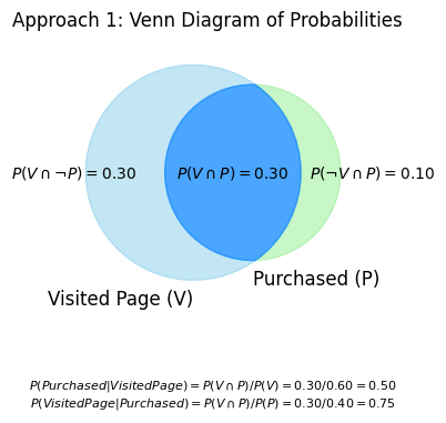
This Venn diagram visually clarifies how different probabilities are related:

• Specific Outcomes: The values inside each distinct segment of the diagram show the probability of that particular, unique scenario occurring. For example:

  • $P(V \cap \neg P)$ represents the probability of a visitor ‘Visiting the Page but Not Purchasing’.

  • $P(V \cap P)$ represents the probability of a visitor ‘Visiting the Page AND Purchasing’.

• Total Event Probabilities: The total probability for an entire event (like ‘Visited Page’, denoted as $P(V)$) is found by summing the probabilities of all the individual segments that make up that event.

  • For instance, $P(V) = P(V \cap \neg P) + P(V \cap P)$.

• Components for Conditional Probability: This total probability (e.g., $P(V)$), along with the probability of the intersection (e.g., $P(V \cap P)$), are the essential values used in the formula for conditional probability.

  • For example, $P(\text{Purchased} | \text{Visited Page}) = P(V \cap P) / P(V)$.

• Visualizing the Sample Space: The diagram effectively helps to see how the entire circle of the conditioning event (e.g., the ‘Visited Page’ circle, representing the total $P(V)$) becomes the new, reduced sample space when calculating a conditional probability.

Approach 2: Direct Conditional Probability¶

• Definition: This approach involves filtering the data to directly calculate the conditional probabilities from the relevant subset of data.

• Calculations:

  • $P(\text{Purchased} \mid \text{Visited Page})$: The DataFrame is filtered to include only visitors who visited the product page. The number of these visitors who made a purchase is then divided by the total number of visitors who visited the page.

  • $P(\text{Visited Page} \mid \text{Purchased})$: The DataFrame is filtered to include only visitors who made a purchase. The number of these visitors who visited the product page is then divided by the total number of visitors who made a purchase.

• Advantage: This method is straightforward and intuitive because it directly uses the relevant subset of data.

# Direct calculation from counts: P(Purchase | Visited Page)
df_visited = df[df['visited_product_page'] == True]
n_purchased_in_visited = df_visited['made_purchase'].sum()
n_visited = len(df_visited)

if n_visited > 0:
    P_purchased_given_visited_direct = n_purchased_in_visited / n_visited
    print(f"Direct P(Purchased | Visited Page) = {P_purchased_given_visited_direct:.2f} ({n_purchased_in_visited}/{n_visited})")
else:
    print("Cannot calculate P(Purchased | Visited Page) directly as no one visited the page.")

# Direct calculation from counts: P(Visited Page | Purchased)
df_purchased = df[df['made_purchase'] == True]
n_visited_in_purchased = df_purchased['visited_product_page'].sum()
n_purchased_total = len(df_purchased)

if n_purchased_total > 0:
    P_visited_given_purchased_direct = n_visited_in_purchased / n_purchased_total
    print(f"Direct P(Visited Page | Purchased) = {P_visited_given_purchased_direct:.2f} ({n_visited_in_purchased}/{n_purchased_total})")
else:
    print("Cannot calculate P(Visited Page | Purchased) directly as no one made a purchase.")

Direct P(Purchased | Visited Page) = 0.50 (3/6)
Direct P(Visited Page | Purchased) = 0.75 (3/4)

import matplotlib.pyplot as plt
import pandas as pd # Added for completeness if you run this standalone with the sample data

# Conceptual Tree Diagram for Approach 2
fig_tree, ax_tree = plt.subplots(figsize=(14, 9)) # Increased size for better readability
ax_tree.set_xlim(0, 10)
ax_tree.set_ylim(0, 10)
ax_tree.axis('off')
ax_tree.text(5, 9.5, "Approach 2: Conceptual Tree Diagram Illustrating Filtering", ha='center', va='center', fontsize=14, weight='bold')

# --- Branch for P(Purchased | Visited Page) ---
ax_tree.text(2.5, 8.5, "$P(Purchased \ | \ Visited \ Page)$", ha='center', va='center', fontsize=12, bbox=dict(facecolor='lightblue', alpha=0.5))
# Root: All Visitors
ax_tree.text(2.5, 7.5, f"All Visitors\n(N={n_total})", ha='center', va='center', bbox=dict(boxstyle="round,pad=0.3", fc="whitesmoke", ec="black"))
# Branch to Visited Page / Not Visited Page
ax_tree.plot([2.5, 1.5], [7.0, 6.0], 'k-')
ax_tree.plot([2.5, 3.5], [7.0, 6.0], 'k-')
ax_tree.text(1.5, 5.5, f"Visited Page (V)\n(N={n_visited_page})", ha='center', va='center', bbox=dict(boxstyle="round,pad=0.3", fc="lightgreen", ec="black", linewidth=2)) # Conditioned on this group
ax_tree.text(3.5, 5.5, f"Not Visited Page (¬V)\n(N={n_total - n_visited_page})", ha='center', va='center', bbox=dict(boxstyle="round,pad=0.3", fc="lightcoral", ec="black"))

# From "Visited Page" (this is the group of size n_visited), branch to Purchased / Not Purchased
ax_tree.text(1.5, 4.8, f"Focus on this group (N={n_visited})", ha='center', va='center', fontsize=9, style='italic', color='darkgreen')
ax_tree.plot([1.5, 0.75], [5.0, 4.0], 'k-') # Line to Purchased
ax_tree.plot([1.5, 2.25], [5.0, 4.0], 'k-') # Line to Not Purchased
ax_tree.text(0.75, 3.5, f"Purchased (P)\n(N={n_purchased_in_visited})", ha='center', va='center', bbox=dict(boxstyle="round,pad=0.3", fc="palegreen", ec="black"))
# Corrected variable: n_visited (length of df_visited)
ax_tree.text(2.25, 3.5, f"Not Purchased (¬P)\n(N={n_visited - n_purchased_in_visited})", ha='center', va='center', bbox=dict(boxstyle="round,pad=0.3", fc="lightpink", ec="black"))
# Corrected variable: n_visited
ax_tree.text(1.5, 2.5, f"$P(P | V) = \\frac{{{n_purchased_in_visited}}}{{{n_visited}}} = {P_purchased_given_visited_direct:.2f}$", ha='center', va='center', fontsize=10, weight='bold', color='darkgreen')


# --- Branch for P(Visited Page | Purchased) ---
ax_tree.text(7.5, 8.5, "$P(Visited \ Page \ | \ Purchased)$", ha='center', va='center', fontsize=12, bbox=dict(facecolor='lightpink', alpha=0.5))
# Root: All Visitors
ax_tree.text(7.5, 7.5, f"All Visitors\n(N={n_total})", ha='center', va='center', bbox=dict(boxstyle="round,pad=0.3", fc="whitesmoke", ec="black"))
# Branch to Purchased / Not Purchased
ax_tree.plot([7.5, 6.5], [7.0, 6.0], 'k-')
ax_tree.plot([7.5, 8.5], [7.0, 6.0], 'k-')
ax_tree.text(6.5, 5.5, f"Purchased (P)\n(N={n_purchased})", ha='center', va='center', bbox=dict(boxstyle="round,pad=0.3", fc="lightgoldenrodyellow", ec="black", linewidth=2)) # Conditioned on this group
ax_tree.text(8.5, 5.5, f"Not Purchased (¬P)\n(N={n_total - n_purchased})", ha='center', va='center', bbox=dict(boxstyle="round,pad=0.3", fc="lightgrey", ec="black"))

# From "Purchased" (this is the group of size n_purchased_total), branch to Visited Page / Not Visited Page
ax_tree.text(6.5, 4.8, f"Focus on this group (N={n_purchased_total})", ha='center', va='center', fontsize=9, style='italic', color='darkred')
ax_tree.plot([6.5, 5.75], [5.0, 4.0], 'k-') # Line to Visited Page
ax_tree.plot([6.5, 7.25], [5.0, 4.0], 'k-') # Line to Not Visited Page
ax_tree.text(5.75, 3.5, f"Visited Page (V)\n(N={n_visited_in_purchased})", ha='center', va='center', bbox=dict(boxstyle="round,pad=0.3", fc="khaki", ec="black"))
# Corrected variable: n_purchased_total (length of df_purchased)
ax_tree.text(7.25, 3.5, f"Not Visited Page (¬V)\n(N={n_purchased_total - n_visited_in_purchased})", ha='center', va='center', bbox=dict(boxstyle="round,pad=0.3", fc="lightgray", ec="black"))
# Corrected variable: n_purchased_total
ax_tree.text(6.5, 2.5, f"$P(V | P) = \\frac{{{n_visited_in_purchased}}}{{{n_purchased_total}}} = {P_visited_given_purchased_direct:.2f}$", ha='center', va='center', fontsize=10, weight='bold', color='darkred')

plt.tight_layout()
plt.show()

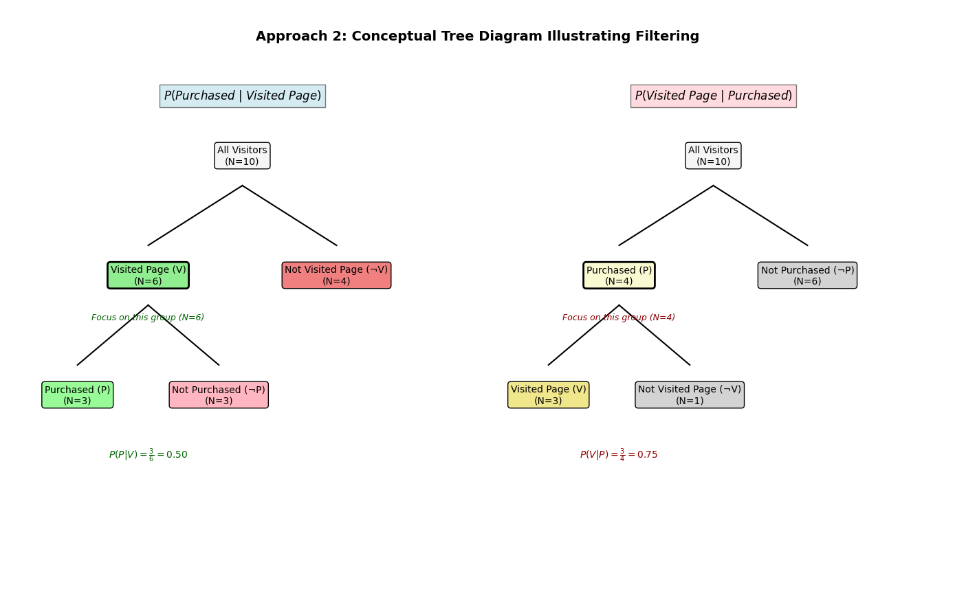
This tree diagram illustrates the direct approach to conditional probability by visually segmenting the visitor population based on a sequence of events or conditions. To find $P(\text{Purchased} | \text{Visited Page})$, for instance, you first follow the branch representing ‘Visited Page’, effectively filtering the data, and then observe the proportion of those visitors who subsequently ‘Made Purchase’. The diagram clearly shows how the initial condition narrows the focus to a specific subgroup before the probability of the second event is determined within that subgroup.

Summary¶

• Calculated Approach: Uses probability rules to derive conditional probabilities from known probabilities.

• Direct Approach: Filters the data to the condition and performs the calculation on the filtered data.

Both approaches should yield the same results if done correctly, and the choice between them can depend on the context and what data or probabilities you already have at hand.

This example shows how to compute conditional probabilities directly from observed data, a common task in data analysis. $P(\text{Purchased} | \text{Visited Page})$ tells us the likelihood of a purchase among those who visited the specific page, while $P(\text{Visited Page} | \text{Purchased})$ tells us the likelihood that someone who did purchase had previously visited that page. These can be very different values!

Applying the Law of Total Probability¶

Let’s use the Law of Total Probability with a manufacturing example. Suppose a factory has two machines, M1 and M2, producing widgets.

• Machine M1 produces 60% of the widgets ($P(M1) = 0.6$).

• Machine M2 produces 40% of the widgets ($P(M2) = 0.4$).

• 2% of widgets from M1 are defective ($P(D|M1) = 0.02$).

• 5% of widgets from M2 are defective ($P(D|M2) = 0.05$).

What is the overall probability that a randomly selected widget is defective ($P(D)$)?

The events M1 (widget produced by M1) and M2 (widget produced by M2) form a partition of the sample space (all widgets). Using the Law of Total Probability:

$P(D) = P(D|M1)P(M1) + P(D|M2)P(M2)$

# Define probabilities
P_M1 = 0.60
P_M2 = 0.40
P_D_given_M1 = 0.02
P_D_given_M2 = 0.05

# Apply Law of Total Probability
P_D = (P_D_given_M1 * P_M1) + (P_D_given_M2 * P_M2)

print(f"P(Defective | M1) = {P_D_given_M1}")
print(f"P(M1) = {P_M1}")
print(f"P(Defective | M2) = {P_D_given_M2}")
print(f"P(M2) = {P_M2}")
print("\n")
print(f"Overall Probability of a Defective Widget P(D) = ({P_D_given_M1} * {P_M1}) + ({P_D_given_M2} * {P_M2}) = {P_D:.4f}")

P(Defective | M1) = 0.02
P(M1) = 0.6
P(Defective | M2) = 0.05
P(M2) = 0.4


Overall Probability of a Defective Widget P(D) = (0.02 * 0.6) + (0.05 * 0.4) = 0.0320

So, the overall probability of finding a defective widget is 3.2%. This weighted average reflects that while M2 produces more defective items proportionatly, M1 produces more items overall.

We could also simulate this:

num_widgets_sim = 100000
defective_count = 0

for _ in range(num_widgets_sim):
    # Decide which machine produced the widget
    if random.random() < P_M1: # Simulates P(M1)
        # Widget from M1
        # Check if it's defective
        if random.random() < P_D_given_M1: # Simulates P(D|M1)
            defective_count += 1
    else:
        # Widget from M2
        # Check if it's defective
        if random.random() < P_D_given_M2: # Simulates P(D|M2)
            defective_count += 1

# Estimate P(D) from simulation
P_D_sim = defective_count / num_widgets_sim

print(f"\n--- Simulation Results ({num_widgets_sim} widgets) ---")
print(f"Estimated overall P(Defective): {P_D_sim:.4f}")

--- Simulation Results (100000 widgets) ---
Estimated overall P(Defective): 0.0314

Again, the simulation provides an estimate very close to the calculated value.

This chapter introduced conditional probability, the multiplication rule, the law of total probability, and tree diagrams. These concepts are crucial for reasoning under uncertainty and form the basis for more advanced topics like Bayes’ Theorem, which we will explore in the next chapter. The hands-on examples demonstrated how to calculate and simulate these probabilities using Python.

Okay, here is the entire “Exercises” section with the questions followed by their respective dropdown explanations: