Chapter 1: Introduction to Probability and Python Setup#
Welcome to “Probability in Practice: A Hands-On Journey with Python”! This first chapter lays the groundwork for our exploration. We’ll start by understanding what probability is and why it’s such a fundamental concept in so many fields. Then, we’ll introduce the essential Python tools we’ll be using throughout the book and guide you through setting up your environment and performing some basic operations.
1.1 What is Probability? Why is it important?#
At its core, probability is the mathematical language we use to describe and quantify uncertainty. It’s a way of measuring the likelihood or chance that a specific event will occur out of a set of possible outcomes. We express probability as a number between 0 and 1, inclusive:
A probability of 0 means the event is impossible.
A probability of 1 means the event is certain.
A probability between 0 and 1 indicates varying degrees of likelihood (e.g., 0.5 means a 50% chance, like a fair coin landing on heads).
Why is probability important?
Uncertainty is inherent in almost every aspect of the world around us. Probability provides a systematic way to reason about, model, and make decisions in the face of this uncertainty. Its applications are vast and span numerous domains:
Science: Modeling quantum mechanics, predicting experimental outcomes, analyzing genetic inheritance.
Engineering: Assessing structural integrity under stress, designing reliable systems, managing communication network traffic.
Finance & Economics: Pricing options and derivatives, managing investment portfolios, forecasting market movements, assessing credit risk.
Medicine: Evaluating the effectiveness of new treatments, understanding disease transmission, interpreting diagnostic tests.
Machine Learning & AI: Building spam filters, training predictive models, designing recommendation systems, quantifying model confidence.
Gaming & Gambling: Calculating odds, developing game strategies.
Everyday Life: Making weather predictions, deciding whether to buy insurance, understanding opinion polls.
Example: Imagine a company considering launching a new product. Market research data provides insights, but it’s not definitive. Probability helps quantify the risk. Based on survey results, competitor analysis, and economic forecasts, the company might estimate: * P(High Success) = 0.2 (20% chance of high sales) * P(Moderate Success) = 0.5 (50% chance of moderate sales) * P(Failure) = 0.3 (30% chance of failure)
These probabilities, combined with potential profits/losses for each scenario, allow the company to make a more informed decision about whether the potential reward justifies the risk.
Throughout this book, we’ll see how probability allows us to move from vague intuition about uncertainty to precise, quantitative analysis, often aided by the computational power of Python.
1.2 Introduction to the Tools#
To embark on our hands-on journey, we need the right tools. We’ll primarily use Python along with several powerful libraries designed for scientific computing, data analysis, and visualization.
Python: A versatile, high-level programming language known for its readability and extensive ecosystem of libraries. It’s an excellent choice for both learning concepts and implementing practical applications.
Jupyter Notebooks: An interactive computing environment that allows you to create and share documents containing live code, equations, visualizations, and narrative text. They are perfect for exploratory analysis, learning step-by-step, and presenting results. We’ll be using Jupyter Notebooks (or compatible environments like JupyterLab, Google Colab, VS Code Notebooks) for all our examples.
NumPy (Numerical Python): The fundamental package for numerical computation in Python. It provides:
A powerful N-dimensional array object (
ndarray).Functions for mathematical operations, linear algebra, random number generation, and more.
The foundation upon which many other scientific libraries are built.
Example: Simulating 10 coin flips (0 for tails, 1 for heads):
import numpy as np
flips = np.random.randint(0, 2, size=10)
print(flips) # Output might be: [0 1 1 0 1 0 0 1 0 1]
Matplotlib & Seaborn: Libraries for data visualization.
Matplotlib: A comprehensive library for creating static, animated, and interactive visualizations. It provides fine-grained control over plots.
Seaborn: Built on top of Matplotlib, Seaborn provides a high-level interface for drawing attractive and informative statistical graphics, often with less code. We’ll use both, leveraging Seaborn for quick, standard plots and Matplotlib for customization.
Example: Creating a simple histogram (we’ll see a full example in the Hands-on section).
SciPy (Scientific Python): A library that builds on NumPy and provides a large collection of algorithms and functions for scientific and technical computing. We will specifically use its
scipy.statsmodule, which contains tools for:Working with a wide range of probability distributions (calculating probabilities, generating random numbers, fitting distributions to data).
Performing statistical tests.
Example: Calculating the probability of getting exactly 3 heads in 5 fair coin flips using the binomial distribution (more on this in later chapters).
Don’t worry if these seem like a lot right now. We’ll introduce functions and concepts from these libraries gradually as needed throughout the book. The key is to get comfortable with the basic environment and operations first.
1.3 Hands-on: Setting up and Basic Operations#
Let’s get our hands dirty! This section walks through setting up your environment and trying out some basic commands.
1.3.1 Setting up the Environment#
The most straightforward way to get Python and the necessary libraries is to install the Anaconda Distribution. Anaconda bundles Python, Jupyter, NumPy, SciPy, Matplotlib, and many other useful scientific libraries into a single, easy-to-install package.
Download Anaconda: Go to the Anaconda Distribution website and download the installer for your operating system (Windows, macOS, Linux).
Install Anaconda: Run the installer, following the on-screen instructions. It’s generally recommended to accept the default settings unless you have specific reasons not to.
Launch Jupyter Notebook/Lab:
Using Anaconda Navigator: Open Anaconda Navigator (which was installed along with Anaconda) and launch “Jupyter Notebook” or “JupyterLab” (JupyterLab is a more modern interface).
Using the Terminal/Command Prompt: Open your terminal (macOS/Linux) or Anaconda Prompt (Windows) and type
jupyter notebookorjupyter laband press Enter.
Your web browser should open, displaying the Jupyter interface, typically showing files in your home directory.
Alternative (using pip): If you already have Python installed and prefer not to use Anaconda, you can install the libraries individually using pip, Python’s package installer. Open your terminal or command prompt and run:
pip install numpy matplotlib seaborn scipy jupyterlab
Then launch JupyterLab by typing jupyter lab in the terminal.
1.3.2 Basic Jupyter Usage#
Jupyter Notebooks consist of cells. The two main types are:
Code cells: Contain Python code that you can execute.
Markdown cells: Contain text, headings, lists, images, and equations formatted using Markdown syntax (like this cell!).
Key Actions:
Running a cell: Select the cell by clicking on it and press
Shift + Enter(or click the “Run” button in the toolbar). This executes the code (if it’s a code cell) or renders the text (if it’s a Markdown cell) and moves to the next cell.Ctrl + Enterruns the cell but stays selected.Changing cell type: Use the dropdown menu in the toolbar to switch between Code and Markdown.
Adding cells: Use the
+button in the toolbar.Saving: Notebooks are saved automatically, but you can force a save with
Ctrl + Sor the save icon.
Try it: Create a new code cell, type print("Hello Probability!"), and run it using Shift + Enter.
print("Hello Probability!")
Hello Probability!
1.3.3 Simple NumPy Array Manipulations#
Let’s create some NumPy arrays and perform basic operations. The standard convention is to import NumPy as np.
import numpy as np
# Create a 1D array (vector) from a list
my_list = [1, 2, 3, 4, 5]
my_array = np.array(my_list)
print("1D Array:", my_array)
print("Type:", type(my_array))
print("Shape:", my_array.shape) # Shape is (5,) meaning 5 elements along one dimension
1D Array: [1 2 3 4 5]
Type: <class 'numpy.ndarray'>
Shape: (5,)
# Create a 2D array (matrix)
my_2d_array = np.array([[1, 2, 3], [4, 5, 6]])
print("\n2D Array:\n", my_2d_array)
print("Shape:", my_2d_array.shape) # Shape is (2, 3) meaning 2 rows, 3 columns
2D Array:
 [[1 2 3]
 [4 5 6]]
Shape: (2, 3)
# Create arrays with specific values
zeros_array = np.zeros((2, 4)) # Array of zeros with shape (2, 4)
print("\nZeros Array:\n", zeros_array)
Zeros Array:
 [[0. 0. 0. 0.]
 [0. 0. 0. 0.]]
ones_array = np.ones(5) # Array of ones with shape (5,)
print("\nOnes Array:", ones_array)
Ones Array: [1. 1. 1. 1. 1.]
# Create arrays with sequences
range_array = np.arange(0, 10, 2) # Like Python's range: start, stop (exclusive), step
print("\nRange Array:", range_array)
Range Array: [0 2 4 6 8]
# Basic arithmetic operations (element-wise)
arr1 = np.array([10, 20, 30])
arr2 = np.array([1, 2, 3])
print("\nArray Addition:", arr1 + arr2)
print("Array Multiplication:", arr1 * arr2)
print("Adding a scalar:", arr1 + 100)
Array Addition: [11 22 33]
Array Multiplication: [10 40 90]
Adding a scalar: [110 120 130]
# Random numbers
# Generate 5 random numbers from a uniform distribution between 0 and 1
random_uniform = np.random.rand(5)
print("\nRandom Uniform:", random_uniform)
Random Uniform: [0.47769972 0.24901336 0.22172112 0.48843462 0.74310397]
# Generate 6 random integers between 1 (inclusive) and 7 (exclusive) - simulating dice rolls
dice_rolls_example = np.random.randint(1, 7, size=6)
print("Simulated Dice Rolls:", dice_rolls_example)
Simulated Dice Rolls: [4 1 3 1 1 3]
1.3.4 Plotting a Basic Graph with Matplotlib#
Visualization is crucial for understanding probability distributions and simulation results. Let’s simulate rolling a standard six-sided die many times and plot a histogram of the outcomes. We expect each outcome (1 through 6) to be roughly equally likely if we perform many rolls.
We’ll use matplotlib.pyplot, conventionally imported as plt.
import matplotlib.pyplot as plt
import numpy as np # Ensure numpy is imported
# --- Simulation Parameters ---
num_rolls = 1000  # Let's simulate rolling the die 1000 times
die_sides = 6
# --- Simulate the Dice Rolls ---
# np.random.randint(low, high, size) generates integers from low (inclusive) to high (exclusive)
rolls = np.random.randint(1, die_sides + 1, size=num_rolls)
# --- Create the Histogram ---
# plt.hist() calculates and draws the histogram
# bins defines the edges of the bins. We want bins [1, 2), [2, 3), ..., [6, 7)
# We use np.arange(1, die_sides + 2) which gives [1, 2, 3, 4, 5, 6, 7]
# align='left' means the bar label corresponds to the left edge (e.g., label '1' for bin [1, 2))
# rwidth controls the relative width of the bars
plt.figure(figsize=(8, 5)) # Optional: sets the figure size
plt.hist(rolls, bins=np.arange(1, die_sides + 2), align='left', rwidth=0.8, color='skyblue', edgecolor='black')

# --- Add Labels and Title ---
plt.title(f'Histogram of {num_rolls} Dice Rolls')
plt.xlabel('Die Outcome')
plt.ylabel('Frequency (Count)')
plt.xticks(np.arange(1, die_sides + 1)) # Set ticks explicitly to 1, 2, ..., 6
plt.grid(axis='y', linestyle='--', alpha=0.7) # Add horizontal grid lines
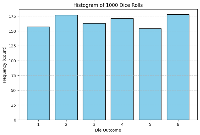
If you run the code cell above, you should see a histogram. Because the rolls are random, the bars won’t be perfectly equal, especially with only 1000 rolls. However, you should observe that the frequencies for each outcome (1 to 6) are roughly similar. As we increase num_rolls (try changing it to 10000 or 100000 and rerunning), the bars should become even closer in height, illustrating the concept of probabilities evening out over many trials (which we’ll formally call the Law of Large Numbers later).
Chapter Summary#
In this chapter, we introduced the fundamental concept of probability as a measure of uncertainty and highlighted its importance across various fields. We also familiarized ourselves with the essential Python toolkit for this book: Jupyter Notebooks, NumPy, Matplotlib, and SciPy. Finally, we walked through setting up the environment and performed basic operations, including array manipulation with NumPy and plotting a histogram with Matplotlib.
You should now have a working Python environment and a basic understanding of how to execute code and visualize simple data within a Jupyter Notebook.
In the next chapter, we will delve into the formal language of probability, defining key terms like sample spaces, events, and outcomes, and exploring the fundamental axioms and rules that govern probability calculations.