Chapter 7: Common Discrete Distributions

In the previous chapter, we defined discrete random variables and learned how to describe their behavior using Probability Mass Functions (PMFs), Cumulative Distribution Functions (CDFs), expected value, and variance. While we can define custom PMFs for any situation, several specific discrete distributions appear so frequently in practice that they have been studied extensively and given names.

These “common” distributions serve as powerful models for a wide variety of real-world processes. Understanding their properties and when to apply them is crucial for probabilistic modeling. In this chapter, we will explore nine fundamental discrete distributions: Bernoulli, Binomial, Geometric, Negative Binomial, Poisson, Hypergeometric, Discrete Uniform, Categorical, and Multinomial.

We’ll examine the scenarios each distribution models, their key characteristics (PMF, mean, variance), and how to work with them efficiently using Python’s scipy.stats library. This library provides tools to calculate probabilities (PMF, CDF), generate random samples, and more, significantly simplifying our practical work.

import numpy as np
from scipy import stats
import matplotlib.pyplot as plt
import os

# Configure plots
plt.style.use('seaborn-v0_8-whitegrid')

1. Bernoulli Distribution¶

The Bernoulli distribution models a single trial with two possible outcomes: “success” (1) or “failure” (0).

Why Start with Something So Simple?

The Bernoulli distribution might seem almost trivially simple—it’s just a single trial with two outcomes! However, it’s incredibly important because:

It’s the fundamental building block: Several key distributions in this chapter (Binomial, Geometric, Negative Binomial) build directly on repeated Bernoulli trials, while Categorical generalizes the Bernoulli distribution to more than two outcomes
Single binary events are everywhere: Many real-world scenarios involve a single yes/no, success/failure, or on/off decision
It establishes key patterns: The $p$ and $(1-p)$ structure appears throughout probability theory
Mathematical note: The Bernoulli distribution is technically just the Binomial distribution with $n=1$ , but we give it its own name because of its foundational importance

Think of it like learning to add before learning to multiply—simple, but essential!

Concrete Example

Suppose you’re conducting a medical screening test for a disease in a high-risk population. Each test either shows positive or negative. From epidemiological data, you know that 30% of individuals in this population test positive.

We model this with a random variable $X$ :

$X = 1$ if the test result is positive (success)
$X = 0$ if the test result is negative (failure)

The probabilities are:

$P(X = 1) = 0.3$ (we call this parameter $p$ )
$P(X = 0) = 0.7$ (which equals $1 - p$ )

The Bernoulli PMF

For any Bernoulli random variable with success probability $p$ , the PMF is:

P(X=k) = \begin{cases} p & \text{if } k=1 \\ 1-p & \text{if } k=0 \\ 0 & \text{otherwise} \end{cases}

(1)

This can also be written compactly as:

P(X = k) = p^k (1-p)^{1-k} \text{ for } k \in \{0, 1\}

(2)

Expanding this for both cases to make it crystal clear:

When k = 1 (success):

\begin{align} P(X=1) &= p^1 (1-p)^{1-1} \\ &= p^1 (1-p)^0 \\ &= p \times 1 \\ &= p \end{align}

(3)

When k = 0 (failure):

\begin{align} P(X=0) &= p^0 (1-p)^{1-0} \\ &= p^0 (1-p)^1 \\ &= 1 \times (1-p) \\ &= 1-p \end{align}

(4)

Let’s verify this works for our example where $p = 0.3$ :

When $k = 1$ : $P(X=1) = (0.3)^1 (0.7)^0 = 0.3 \times 1 = 0.3$ ✓
When $k = 0$ : $P(X=0) = (0.3)^0 (0.7)^1 = 1 \times 0.7 = 0.7$ ✓

Key Characteristics

Scenarios: Coin flip (Heads/Tails), product inspection (Defective/Not Defective), medical test (Positive/Negative), free throw (Make/Miss)
Parameter: $p$ , the probability of success ( $0 \le p \le 1$ )
Random Variable: $X \in \{0, 1\}$

Mean: $E[X] = p$

Variance: $Var(X) = p(1-p)$

Standard Deviation: $SD(X) = \sqrt{p(1-p)}$

Visualizing the Distribution

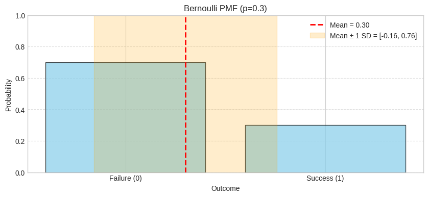
Let’s visualize a Bernoulli distribution with $p = 0.3$ (our medical test example from above):

# Remove existing SVG if present
if os.path.exists('ch07_bernoulli_pmf_generic.svg'):
    os.remove('ch07_bernoulli_pmf_generic.svg')

# Create Bernoulli distribution for visualization (p=0.3)
p_viz = 0.3
bernoulli_viz = stats.bernoulli(p=p_viz)

# Calculate mean and std
mean_viz = bernoulli_viz.mean()
std_viz = bernoulli_viz.std()

# Plotting the PMF
k_values_viz = [0, 1]
pmf_values_viz = bernoulli_viz.pmf(k_values_viz)

plt.figure(figsize=(10, 4))
plt.bar(k_values_viz, pmf_values_viz, tick_label=["Failure (0)", "Success (1)"], color='skyblue', edgecolor='black', alpha=0.7)

# Add mean line
plt.axvline(mean_viz, color='red', linestyle='--', linewidth=2, label=f'Mean = {mean_viz:.2f}')

# Add mean ± 1 std region
plt.axvspan(mean_viz - std_viz, mean_viz + std_viz, alpha=0.2, color='orange',
            label=f'Mean ± 1 SD = [{mean_viz - std_viz:.2f}, {mean_viz + std_viz:.2f}]')

plt.title(f"Bernoulli PMF (p={p_viz})")
plt.xlabel("Outcome")
plt.ylabel("Probability")
plt.ylim(0, 1)
plt.legend(loc='upper right', fontsize=10)
plt.grid(axis='y', linestyle='--', alpha=0.6)
plt.savefig('ch07_bernoulli_pmf_generic.svg', format='svg', bbox_inches='tight')
plt.show()

The PMF shows two bars: P(X=0) = 0.7 for a negative test and P(X=1) = 0.3 for a positive test. The red dashed line marks the mean ( $p = 0.3$ ), and the orange shaded region shows mean ± 1 standard deviation.

# Remove existing SVG if present
if os.path.exists('ch07_bernoulli_cdf_generic.svg'):
    os.remove('ch07_bernoulli_cdf_generic.svg')

# Plotting the CDF
k_values_viz = [0, 1]
cdf_values_viz = bernoulli_viz.cdf(k_values_viz)

plt.figure(figsize=(10, 4))
# Add points to show the full step function including the start at 0
plt.step([-0.5] + k_values_viz, [0] + list(cdf_values_viz), where='post', color='darkgreen', linewidth=2)

# Add mean line
plt.axvline(mean_viz, color='red', linestyle='--', linewidth=2, label=f'Mean = {mean_viz:.2f}')

plt.title(f"Bernoulli CDF (p={p_viz})")
plt.xlabel("Outcome")
plt.ylabel("Cumulative Probability P(X <= k)")
plt.ylim(0, 1.1)
plt.xlim(-0.5, 1.5)
plt.xticks([0, 1])
plt.legend(loc='lower right', fontsize=10)
plt.grid(True, which='both', linestyle='--', linewidth=0.5, alpha=0.6)
plt.savefig('ch07_bernoulli_cdf_generic.svg', format='svg', bbox_inches='tight')
plt.show()

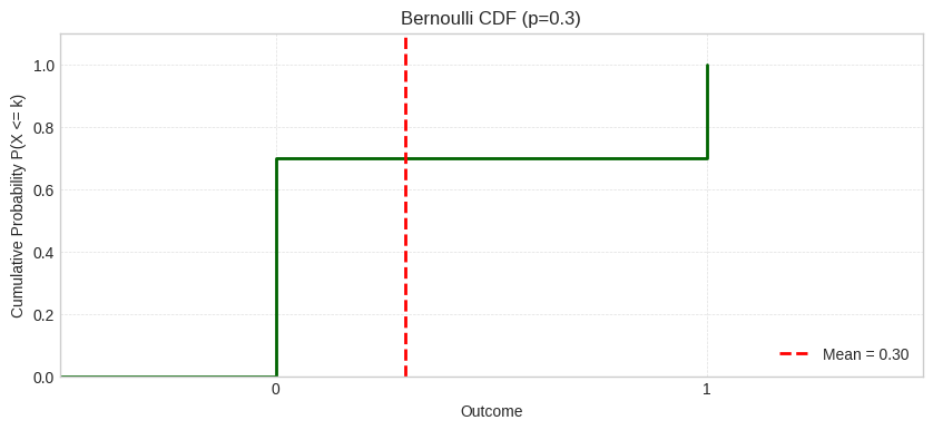
The CDF shows the step function: starts at 0 for x < 0, jumps to 0.7 at x=0 (the value when outcome is 0), stays flat at 0.7 until x=1, then jumps to 1.0 at x=1 (the value when including both outcomes 0 and 1). The red dashed line marks the mean.

Note: Here, P(X ≤ 0) = P(X = 0) = 0.7 because X can’t take negative values; in general, “X ≤ 0” means “at or below 0”, not “exactly 0”.

Reading the PMF

What it shows: The height of each bar represents the probability of that exact outcome
How to read: Look at the bar height to find P(X = k) for any specific value k
Practical use: Answer questions like “What’s the probability of success?” or “What’s the probability of exactly 1 positive test?”
Key property: All bar heights must sum to 1.0 (total probability)
Visualization aids: The red dashed line marks the mean (expected value), and the orange shaded region shows mean ± 1 standard deviation (where ~68% of values typically fall)

Reading the CDF

What it shows: The cumulative probability P(X ≤ k) up to and including each value k
How to read: The height at position k tells you the probability of getting k or fewer successes
Why step functions? For discrete distributions, probability accumulates in jumps at each possible value. Between possible values, the CDF stays constant (no additional probability)
Key identity: The jump at k equals P(X = k) — the size of each step up is the PMF value
Practical uses:
- Find P(X ≤ k) directly by reading the height at k
- Find P(X > k) by calculating 1 - P(X ≤ k)
- Find P(a < X ≤ b) by calculating P(X ≤ b) - P(X ≤ a)
Key property: The CDF is right-continuous, always increases (or stays flat), and approaches 1.0
Visualization aids: The red dashed line marks the mean (expected value) as a reference point

Note on CDF visualization: The charts use where='post' in the step plot to create proper right-continuous step functions. This means the CDF jumps up at each value and includes that value in the cumulative probability.

Example: Medical Diagnostic Test with p = 0.1

Modeling the outcome of a single medical diagnostic test where the probability of a positive result is 0.1.

Let’s use scipy.stats.bernoulli to calculate probabilities, compute the mean and variance, and generate random samples.

import numpy as np
from scipy import stats
import matplotlib.pyplot as plt

# Using scipy.stats.bernoulli
p_positive = 0.1
bernoulli_rv = stats.bernoulli(p=p_positive)

# PMF: Probability of success (k=1) and failure (k=0)
print(f"P(X=1) (Positive Test): {bernoulli_rv.pmf(1):.2f}")
print(f"P(X=0) (Negative Test): {bernoulli_rv.pmf(0):.2f}")

# Mean and Variance
print(f"Mean (Expected Value): {bernoulli_rv.mean():.2f}")
print(f"Variance: {bernoulli_rv.var():.2f}")

P(X=1) (Positive Test): 0.10
P(X=0) (Negative Test): 0.90
Mean (Expected Value): 0.10
Variance: 0.09

Working with Frozen Random Variables in scipy.stats

When we write bernoulli_rv = stats.bernoulli(p=p_positive), we’re creating a frozen random variable — a distribution object with parameters locked in.

Think of it like partial immutability: Similar to how Python’s immutable objects (strings, tuples) can’t be changed after creation, a frozen RV’s distribution parameters are fixed and can’t be modified. The difference is that frozen RVs only “freeze” the parameters (like p=0.1), not the entire object.

Two ways to use scipy.stats:

Non-frozen (pass parameters every time):

stats.bernoulli.pmf(1, p=0.1)
stats.bernoulli.cdf(0, p=0.1)
stats.bernoulli.mean(p=0.1)

Frozen (set parameters once, reuse):

rv = stats.bernoulli(p=0.1)  # Create frozen RV
rv.pmf(1)                     # Use it multiple times
rv.cdf(0)
rv.mean()

Benefits of frozen RVs:

Cleaner, more readable code
More efficient (parameters validated once)
Easier to pass distributions to functions
Matches the pattern in scipy documentation

Throughout this chapter, we use frozen RVs for all examples. This is the recommended approach when working with the same distribution parameters multiple times.

# Generate random samples
n_samples = 10
samples = bernoulli_rv.rvs(size=n_samples)
print(f"{n_samples} simulated test outcomes (1=Positive, 0=Negative):")
print(samples)

10 simulated test outcomes (1=Positive, 0=Negative):
[0 1 0 0 0 0 0 0 0 0]

# Plotting the PMF
k_values = [0, 1]
pmf_values = bernoulli_rv.pmf(k_values)

plt.figure(figsize=(8, 3.5))
plt.bar(k_values, pmf_values, tick_label=["Negative (0)", "Positive (1)"], color='skyblue', edgecolor='black', alpha=0.7)
plt.title(f"Bernoulli PMF (p={p_positive})")
plt.xlabel("Outcome")
plt.ylabel("Probability")
plt.ylim(0, 1)
plt.grid(axis='y', linestyle='--', alpha=0.6)
plt.show()

The PMF shows the probability of each outcome. With p = 0.1, “Negative” has probability 0.9 and “Positive” has probability 0.1.

# Plotting the CDF
cdf_values = bernoulli_rv.cdf(k_values)

plt.figure(figsize=(8, 3.5))
# Add points to show the full step function including the start at 0
plt.step([-0.5] + k_values, [0] + list(cdf_values), where='post', color='darkgreen', linewidth=2)
plt.title(f"Bernoulli CDF (p={p_positive})")
plt.xlabel("Outcome")
plt.ylabel("Cumulative Probability P(X <= k)")
plt.ylim(0, 1.1)
plt.xlim(-0.5, 1.5)
plt.xticks([0, 1])
plt.grid(True, which='both', linestyle='--', linewidth=0.5, alpha=0.6)
plt.show()

The CDF shows the step function: starts at 0 for x < 0, jumps to 0.9 at x=0, stays flat at 0.9 until x=1, then jumps to 1.0 at x=1.

Quick Check Questions

A quality control inspector checks a single product. It’s either defective or not defective. Is this scenario well-modeled by a Bernoulli distribution? Why or why not?

Answer

Yes - This scenario perfectly fits the Bernoulli distribution requirements:

Single trial: Checking one product
Two possible outcomes: Defective (success/1) or not defective (failure/0)
Fixed probability: The defect rate is constant for each product

If the defect rate is 5%, we’d use Bernoulli(p=0.05).

For a Bernoulli distribution with p = 0.3, what is P(X = 0)?

Answer

P(X = 0) = 1 - p = 0.7 - The probability of failure is 1 - p.

A basketball player has a 75% free throw success rate. If we model a single free throw as a Bernoulli trial, what are the mean and variance?

Answer

Mean = 0.75, Variance = 0.75 × 0.25 = 0.1875

Using the formulas E[X] = p and Var(X) = p(1-p):

E[X] = 0.75
Var(X) = 0.75 × (1 - 0.75) = 0.75 × 0.25 = 0.1875

You roll a six-sided die once. Is this well-modeled by a Bernoulli distribution?

Answer

No - A Bernoulli distribution requires exactly two possible outcomes. A die roll has 6 outcomes (1, 2, 3, 4, 5, 6), so Bernoulli doesn’t apply directly.

However, you could use Bernoulli if you redefined the experiment with a binary outcome:

“Does the die show a 6?” (Yes/No) → Bernoulli with p = 1/6
“Is the result even?” (Yes/No) → Bernoulli with p = 1/2

The key: Bernoulli requires exactly two outcomes.

True or False: A Bernoulli random variable can only take on the values 0 and 1.

Answer

True - By definition, a Bernoulli random variable X ∈ {0, 1}, where:

X = 1 represents “success” with probability p
X = 0 represents “failure” with probability 1-p

These are the only two possible outcomes.

2. Binomial Distribution¶

The Binomial distribution models the number of successes in a fixed number of independent Bernoulli trials, where each trial has the same probability of success.

Concrete Example

Suppose you flip a fair coin 10 times. Each flip is a Bernoulli trial with p = 0.5 (probability of heads). How many heads will you get?

We model this with a random variable $X$ :

$X$ = the number of heads in 10 flips
$X$ can take values 0, 1, 2, ..., 10

The probabilities are:

$P(X = 0)$ = probability of 0 heads (all tails)
$P(X = 5)$ = probability of exactly 5 heads
$P(X = 10)$ = probability of 10 heads (all heads)

The Binomial PMF

For $n$ independent trials with success probability $p$ :

P(X=k) = \binom{n}{k} p^k (1-p)^{n-k}

(5)

for $k = 0, 1, \dots, n$

where $\binom{n}{k} = \frac{n!}{k!(n-k)!}$ is the binomial coefficient (number of ways to choose $k$ successes from $n$ trials).

Understanding the Binomial Formula

The Binomial PMF formula combines probability and counting:

P(X=k) = \binom{n}{k} \cdot p^k \cdot (1-p)^{n-k}

(6)

Breaking down the formula:

$p^k$ : Probability of $k$ successes — each success is an independent Bernoulli trial with probability $p$
$(1-p)^{n-k}$ : Probability of $(n-k)$ failures — each failure is an independent Bernoulli trial with probability $1-p$
$\binom{n}{k}$ : Number of ways to arrange $k$ successes among $n$ trial positions

The probabilistic view (Bernoulli trials):

Any specific sequence of $k$ successes and $(n-k)$ failures has probability $p^k(1-p)^{n-k}$ (by independence of trials). For example, the sequence “success, success, failure” has probability $p \cdot p \cdot (1-p) = p^2(1-p)$ .

This shows why Binomial “counts successes in repeated Bernoulli trials”: it’s built from the ground up using the Bernoulli probability $p$ for each trial.

The combinatorial view (counting techniques):

The binomial coefficient $\binom{n}{k}$ is a combination that counts the number of ways to choose $k$ items from $n$ items when order doesn’t matter (see Chapter 3: Combinations).

In our context, it counts how many different sequences of $n$ trials yield exactly $k$ successes. For example, with $n=3$ trials and $k=2$ successes: $\binom{3}{2} = 3$ represents the three sequences SSF, SFS, and FSS (where S=success, F=failure).

Why we multiply: Each of the $\binom{n}{k}$ sequences has the same probability $p^k(1-p)^{n-k}$ . To get the total probability of exactly $k$ successes (in any order), we multiply the number of sequences by the probability of each sequence.

Visual example: Here’s how it works for $n=3$ trials, $k=2$ successes, with $p=0.6$ :

# Remove existing SVG if present
if os.path.exists('ch07_binomial_formula_breakdown.svg'):
    os.remove('ch07_binomial_formula_breakdown.svg')

import matplotlib.pyplot as plt
from matplotlib.patches import FancyBboxPatch

# --- Parameters ---
n, k, p = 3, 2, 0.6
q = 1 - p
prob_each = (p**k) * (q**(n-k))
total = 3 * prob_each

fig, ax = plt.subplots(figsize=(14, 8), constrained_layout=True)
ax.set_axis_off()
ax.set_xlim(0, 1)
ax.set_ylim(0, 1)

# ---------------- helpers ----------------
def rounded_box(ax, xy, w, h, fc, ec, lw=2, pad=0.012, r=0.02, z=3):
    x, y = xy
    patch = FancyBboxPatch(
        (x, y), w, h,
        boxstyle=f"round,pad={pad},rounding_size={r}",
        transform=ax.transAxes,
        facecolor=fc, edgecolor=ec, linewidth=lw, zorder=z
    )
    ax.add_patch(patch)
    return patch

def draw_sequence(ax, cx, cy, label):
    w, h = 0.14, 0.075
    rounded_box(ax, (cx - w/2, cy - h/2), w, h,
                fc="lightblue", ec="steelblue", lw=2.2, r=0.02)

    ax.text(cx, cy, label, transform=ax.transAxes,
            ha="center", va="center",
            fontsize=24, weight="bold", family="monospace", zorder=4)

    ax.text(cx, cy - 0.075, rf"${p:.1f}\times{p:.1f}\times{q:.1f}$",
            transform=ax.transAxes, ha="center", va="top",
            fontsize=18, zorder=4)

    ax.text(cx, cy - 0.115, rf"$= {prob_each:.3f}$",
            transform=ax.transAxes, ha="center", va="top",
            fontsize=18, weight="bold", zorder=4)

    # return (left, bottom, right, top) for arrow anchoring
    return (cx - w/2, cy - h/2, cx + w/2, cy + h/2)

# ---------------- layout ----------------
ax.text(0.5, 0.955, rf"Binomial Formula Breakdown: $n={n},\,k={k},\,p={p}$",
        transform=ax.transAxes, ha="center", va="top",
        fontsize=24, weight="bold", zorder=4)

# Top row: sequences
seq_y = 0.78
seq_boxes = {}
for lbl, x in [("SSF", 0.24), ("SFS", 0.50), ("FSS", 0.76)]:
    seq_boxes[lbl] = draw_sequence(ax, x, seq_y, lbl)

# Count box
count_w, count_h = 0.30, 0.08
count_xy = (0.5 - count_w/2, 0.56 - count_h/2)
rounded_box(ax, count_xy, count_w, count_h,
            fc="lightyellow", ec="orange", lw=2.2, r=0.02)

ax.text(0.5, 0.56, r"$\binom{3}{2}=3$ sequences",
        transform=ax.transAxes, ha="center", va="center",
        fontsize=20, weight="bold", zorder=4)

# Formula block
ax.text(0.5, 0.44, "Formula:", transform=ax.transAxes,
        ha="center", va="center", fontsize=20, weight="bold", zorder=4)

ax.text(0.5, 0.385, r"$P(X=2)=\binom{3}{2}\cdot p^2\cdot (1-p)^1$",
        transform=ax.transAxes, ha="center", va="center", fontsize=18, zorder=4)

ax.text(0.5, 0.33, r"$=3\times 0.36\times 0.4$",
        transform=ax.transAxes, ha="center", va="center", fontsize=18, zorder=4)

# Result box (moved DOWN a bit)
res_w, res_h = 0.18, 0.075
res_center_y = 0.235  # was 0.26
res_xy = (0.5 - res_w/2, res_center_y - res_h/2)
rounded_box(ax, res_xy, res_w, res_h,
            fc="lightgreen", ec="green", lw=2.2, r=0.02)

ax.text(0.5, res_center_y, rf"$= {total:.3f}$",
        transform=ax.transAxes, ha="center", va="center",
        fontsize=20, weight="bold", zorder=4)

# ---- Callouts: arrows hit box edges and avoid overlaps ----
# Orange (label moved down a bit)
count_tip = (count_xy[0], count_xy[1] + count_h*0.55)  # left edge of yellow box
ax.annotate("Count sequences",
            xy=count_tip, xycoords=ax.transAxes,
            xytext=(0.08, 0.595), textcoords=ax.transAxes,  # moved down
            arrowprops=dict(arrowstyle="->",
                            connectionstyle="arc3,rad=-0.10",
                            lw=2.5, color="orange",
                            shrinkA=6, shrinkB=8),
            fontsize=16, color="orange", weight="bold",
            ha="left", va="center", zorder=5)

# Blue -> right edge of FSS box
x0, y0, x1, y1 = seq_boxes["FSS"]
fss_tip = (x1, (y0 + y1) / 2)
ax.annotate("Each sequence\nhas same\nprobability",
            xy=fss_tip, xycoords=ax.transAxes,
            xytext=(0.88, 0.84), textcoords=ax.transAxes,
            arrowprops=dict(arrowstyle="->",
                            connectionstyle="arc3,rad=0.18",
                            lw=2.5, color="steelblue",
                            shrinkA=6, shrinkB=10),
            fontsize=16, color="steelblue", weight="bold",
            ha="left", va="center", zorder=5)

# Green -> right edge of result box
res_tip = (res_xy[0] + res_w, res_xy[1] + res_h*0.55)
ax.annotate("Multiply!",
            xy=res_tip, xycoords=ax.transAxes,
            xytext=(0.78, 0.19), textcoords=ax.transAxes,  # nudged down
            arrowprops=dict(arrowstyle="->",
                            connectionstyle="arc3,rad=0.10",
                            lw=2.5, color="green",
                            shrinkA=6, shrinkB=10),
            fontsize=16, color="green", weight="bold",
            ha="left", va="center", zorder=5)

# Bottom explanation
why = (
    f"Why it works: Each sequence occurs with probability {total:.3f}/3 = {prob_each:.3f}, "
    f"and there are 3 ways to get exactly 2 successes, so total = 3 × {prob_each:.3f} = {total:.3f}."
)
ax.text(0.5, 0.10, why,
        transform=ax.transAxes, ha="center", va="center",
        fontsize=14, style="italic", wrap=True, zorder=4)

plt.savefig('ch07_binomial_formula_breakdown.svg', format='svg', bbox_inches='tight')
plt.show()

The diagram shows how the formula components work together: we count the sequences (3), calculate the probability of each sequence (0.144), and multiply to get the total probability of exactly 2 successes (0.432).

Let’s verify this works for our coin flip example (n=10, p=0.5):

\begin{align} P(X=5) &= \binom{10}{5} p^5 (1-p)^{10-5} \\ &= \binom{10}{5} (0.5)^5 (1-0.5)^5 \\ &= \binom{10}{5} (0.5)^5 (0.5)^5 \\ &= 252 \times 0.03125 \times 0.03125 \\ &\approx 0.246 \quad \checkmark \end{align}

(7)

Key Characteristics

Scenarios: Number of heads in coin flips, defective items in a batch, successful free throws, correct guesses on a test, customers who purchase
Parameters:
- $n$ : number of independent trials
- $p$ : probability of success on each trial ( $0 \le p \le 1$ )
Random Variable: $X \in \{0, 1, 2, ..., n\}$

Mean: $E[X] = np$

Variance: $Var(X) = np(1-p)$

Standard Deviation: $SD(X) = \sqrt{np(1-p)}$

Visualizing the Distribution

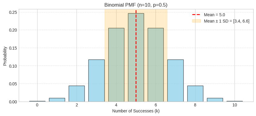
Let’s visualize a Binomial distribution with $n = 10$ and $p = 0.5$ (our coin flip example):

# Remove existing SVG if present
if os.path.exists('ch07_binomial_pmf_generic.svg'):
    os.remove('ch07_binomial_pmf_generic.svg')

# Create Binomial distribution for visualization (n=10, p=0.5)
n_viz = 10
p_viz = 0.5
binomial_viz = stats.binom(n=n_viz, p=p_viz)

# Calculate mean and std
mean_viz = binomial_viz.mean()
std_viz = binomial_viz.std()

# Plotting the PMF
k_values_viz = np.arange(0, n_viz + 1)
pmf_values_viz = binomial_viz.pmf(k_values_viz)

plt.figure(figsize=(10, 4))
plt.bar(k_values_viz, pmf_values_viz, color='skyblue', edgecolor='black', alpha=0.7)

# Add mean line
plt.axvline(mean_viz, color='red', linestyle='--', linewidth=2, label=f'Mean = {mean_viz:.1f}')

# Add mean ± 1 std region
plt.axvspan(mean_viz - std_viz, mean_viz + std_viz, alpha=0.2, color='orange',
            label=f'Mean ± 1 SD = [{mean_viz - std_viz:.1f}, {mean_viz + std_viz:.1f}]')

plt.title(f"Binomial PMF (n={n_viz}, p={p_viz})")
plt.xlabel("Number of Successes (k)")
plt.ylabel("Probability")
plt.legend(loc='upper right', fontsize=10)
plt.grid(axis='y', linestyle='--', alpha=0.6)
plt.savefig('ch07_binomial_pmf_generic.svg', format='svg', bbox_inches='tight')
plt.show()

The PMF shows the probability distribution for the number of heads in 10 coin flips. The distribution is symmetric around the mean ( $np = 5$ ) since $p = 0.5$ . The shaded region shows mean ± 1 standard deviation ( $\sqrt{np(1-p)} = \sqrt{2.5} \approx 1.58$ ).

# Remove existing SVG if present
if os.path.exists('ch07_binomial_cdf_generic.svg'):
    os.remove('ch07_binomial_cdf_generic.svg')

# Plotting the CDF
cdf_values_viz = binomial_viz.cdf(k_values_viz)

plt.figure(figsize=(10, 4))
plt.step(k_values_viz, cdf_values_viz, where='post', color='darkgreen', linewidth=2)

# Add mean line
plt.axvline(mean_viz, color='red', linestyle='--', linewidth=2, label=f'Mean = {mean_viz:.1f}')

plt.title(f"Binomial CDF (n={n_viz}, p={p_viz})")
plt.xlabel("Number of Successes (k)")
plt.ylabel("Cumulative Probability P(X <= k)")
plt.legend(loc='lower right', fontsize=10)
plt.grid(True, which='both', linestyle='--', linewidth=0.5, alpha=0.6)
plt.savefig('ch07_binomial_cdf_generic.svg', format='svg', bbox_inches='tight')
plt.show()

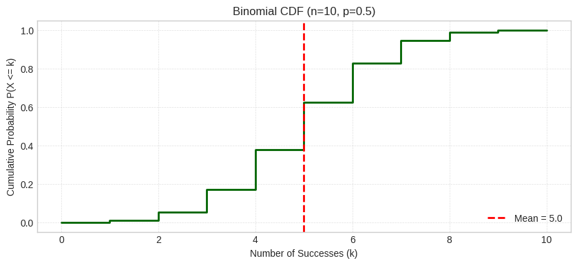
The CDF shows P(X ≤ k), the cumulative probability of getting k or fewer heads. The red dashed line marks the mean.

Example: Sales Calls with n = 20, p = 0.15

Modeling the number of successful sales calls out of 20, where each call has a 0.15 probability of success.

We’ll demonstrate how to use scipy.stats.binom to calculate probabilities, compute statistics, and generate random samples.

Setting up the distribution:

We create a binomial distribution object with our parameters (20 trials, 0.15 success probability):

import numpy as np
from scipy import stats
import matplotlib.pyplot as plt

# Using scipy.stats.binom
n_calls = 20
p_success_call = 0.15
binomial_rv = stats.binom(n=n_calls, p=p_success_call)

Calculating specific probabilities using the PMF:

What’s the probability of getting exactly 5 successful sales out of 20 calls?

# PMF: Probability of exactly k successes
k_successes = 5
print(f"P(X={k_successes} successes out of {n_calls}): {binomial_rv.pmf(k_successes):.4f}")

P(X=5 successes out of 20): 0.1028

With a 10.23% probability, 5 successes is reasonably likely but not the most probable outcome (the mode is at 3 successes, matching the mean of np = 20 × 0.15 = 3).

Calculating cumulative probabilities using the CDF:

What’s the probability of getting 3 or fewer successes? Or more than 3?

# CDF: Probability of k or fewer successes
k_or_fewer = 3
print(f"P(X <= {k_or_fewer} successes out of {n_calls}): {binomial_rv.cdf(k_or_fewer):.4f}")
print(f"P(X > {k_or_fewer} successes out of {n_calls}): {1 - binomial_rv.cdf(k_or_fewer):.4f}")
print(f"P(X > {k_or_fewer} successes out of {n_calls}) (using sf): {binomial_rv.sf(k_or_fewer):.4f}")

P(X <= 3 successes out of 20): 0.6477
P(X > 3 successes out of 20): 0.3523
P(X > 3 successes out of 20) (using sf): 0.3523

There’s a 64.85% chance of getting 3 or fewer successes, meaning there’s a 35.15% chance of getting more than 3 successes.

Note on Survival Function (sf): The sf() method computes the survival function, which is P(X > k) = 1 - P(X ≤ k). While mathematically equivalent to 1 - cdf(k), using sf(k) directly is preferable because it provides better numerical accuracy when dealing with very small or very large probabilities, and makes the code’s intent clearer.

Computing mean and variance:

Let’s verify the theoretical formulas E[X] = np and Var(X) = np(1-p):

# Mean and Variance
print(f"Mean (Expected number of successes): {binomial_rv.mean():.2f}")
print(f"Variance: {binomial_rv.var():.2f}")
print(f"Standard Deviation: {binomial_rv.std():.2f}")

Mean (Expected number of successes): 3.00
Variance: 2.55
Standard Deviation: 1.60

As expected, we get a mean of 3.00 successes (20 × 0.15) with a standard deviation of about 1.6, indicating moderate variability around the mean.

Generating random samples:

We can simulate many rounds of 20 sales calls to see the distribution of outcomes:

# Generate random samples
n_simulations = 1000
samples = binomial_rv.rvs(size=n_simulations)
# print(f"\nSimulated number of successes in {n_calls} calls ({n_simulations} simulations): {samples[:20]}...") # Print first 20

These samples represent 1000 different salespeople each making 20 calls, showing the natural variation in outcomes.

Visualizing the PMF:

Let’s see the complete probability distribution across all possible outcomes (0 to 20 successes):

# Plotting the PMF
k_values = np.arange(0, n_calls + 1)
pmf_values = binomial_rv.pmf(k_values)

plt.figure(figsize=(8, 3.5))
plt.bar(k_values, pmf_values, color='skyblue', edgecolor='black', alpha=0.7)
plt.title(f"Binomial PMF (n={n_calls}, p={p_success_call})")
plt.xlabel("Number of Successes (k)")
plt.ylabel("Probability")
plt.grid(axis='y', linestyle='--', alpha=0.6)
plt.show()

The PMF shows the probability distribution for the number of successful calls. With n = 20 and p = 0.15, the distribution is centered around np = 3 successes (the peak). The distribution is slightly right-skewed because p < 0.5. Notice that getting 0, 1, or 2 successes is quite likely, while getting more than 8 successes is very unlikely.

Visualizing the CDF:

The cumulative distribution shows how probability accumulates as we move from 0 to 20 successes:

# Plotting the CDF
cdf_values = binomial_rv.cdf(k_values)

plt.figure(figsize=(8, 3.5))
plt.step(k_values, cdf_values, where='post', color='darkgreen', linewidth=2)
plt.title(f"Binomial CDF (n={n_calls}, p={p_success_call})")
plt.xlabel("Number of Successes (k)")
plt.ylabel("Cumulative Probability P(X <= k)")
plt.grid(True, which='both', linestyle='--', linewidth=0.5, alpha=0.6)
plt.show()

The CDF shows P(X ≤ k), the cumulative probability of getting k or fewer successful calls. We can see that P(X ≤ 3) ≈ 0.65 (matching our earlier calculation), and by k = 8, we’ve accumulated nearly all the probability (close to 1.0).

Quick Check Questions

You roll a die 12 times and count how many times you get a 6. Is this a good fit for the Binomial distribution? Why or why not?

Answer

Yes, this is a good fit for Binomial. It satisfies all the requirements: (1) fixed number of trials (n = 12 rolls), (2) each trial is independent, (3) only two outcomes per trial (rolling a 6 vs not rolling a 6), and (4) constant success probability (p = 1/6 for each roll). The parameters would be n = 12 and p = 1/6.

For a Binomial distribution with n = 8 and p = 0.25, what is the expected value (mean)?

Answer

E[X] = np = 8 × 0.25 = 2 - The expected number of successes in 8 trials is 2.

A basketball player has a 70% free throw success rate. You watch her take 15 free throws. Does this scenario fit the Binomial distribution assumptions?

Answer

Yes, this fits the Binomial distribution with n = 15 and p = 0.7. Each free throw is independent, has two outcomes (make or miss), and the success probability remains constant at 0.7 for each attempt. We can use this to calculate probabilities like “What’s the chance she makes at least 12 out of 15?”

For a Binomial(n=20, p=0.3) distribution, what is the variance?

Answer

Var(X) = np(1-p) = 20 × 0.3 × 0.7 = 4.2

Using the variance formula for Binomial distributions.

True or False: In a Binomial distribution, each trial must have the same probability of success.

Answer

True - The Binomial distribution requires:

Fixed number of independent trials (n)
Each trial has only two outcomes (success/failure)
Constant success probability (p) across all trials
Trials are independent

If the success probability changes from trial to trial, Binomial doesn’t apply.

3. Geometric Distribution¶

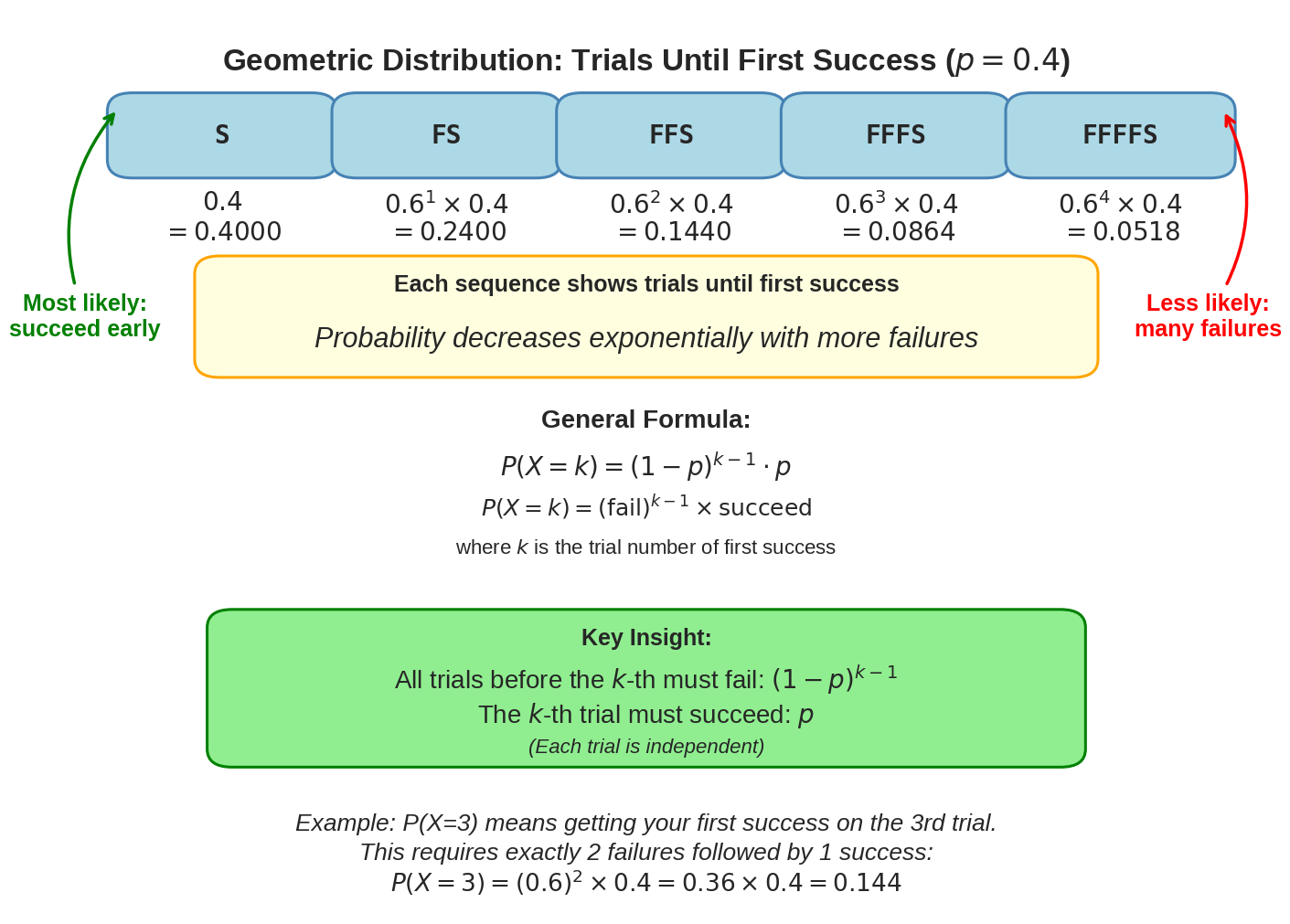
The Geometric distribution models the number of independent Bernoulli trials needed to get the first success.

Concrete Example

You’re shooting free throws until you make your first basket. Each shot has a 0.4 probability of success. How many shots will it take to make your first basket?

We model this with a random variable $X$ :

$X$ = the trial number on which the first success occurs
$X$ can take values 1, 2, 3, ... (first shot, second shot, etc.)

The probabilities are:

$P(X = 1)$ = make it on first shot = 0.4
$P(X = 2)$ = miss first, make second = $(1-0.4) \times 0.4 = 0.24$
$P(X = 3)$ = miss first two, make third = $(1-0.4)^2 \times 0.4 = 0.144$

The Geometric PMF

For trials with success probability $p$ :

P(X=k) = (1-p)^{k-1} p

(8)

for $k = 1, 2, 3, \dots$

This means $k-1$ failures followed by one success.

Let’s verify for our example (p=0.4):

$P(X=2) = (0.6)^1 (0.4) = 0.24$ ✓

Visual example: Here’s how the geometric distribution works with $p=0.4$ (our free throw example):

# Remove existing SVG if present
if os.path.exists('ch07_geometric_formula_breakdown.svg'):
    os.remove('ch07_geometric_formula_breakdown.svg')

import matplotlib.pyplot as plt
from matplotlib.patches import FancyBboxPatch

# --- Parameters ---
p = 0.4
q = 1 - p  # 0.6

fig, ax = plt.subplots(figsize=(14, 10), constrained_layout=True)
ax.set_axis_off()
ax.set_xlim(0, 1)
ax.set_ylim(0, 1)

# ---------------- helpers ----------------
def rounded_box(ax, xy, w, h, fc, ec, lw=2, pad=0.012, r=0.02, z=3):
    x, y = xy
    patch = FancyBboxPatch(
        (x, y), w, h,
        boxstyle=f"round,pad={pad},rounding_size={r}",
        transform=ax.transAxes,
        facecolor=fc, edgecolor=ec, linewidth=lw, zorder=z
    )
    ax.add_patch(patch)
    return patch

def draw_sequence(ax, cx, cy, label, k, prob_val):
    w, h = 0.16, 0.07
    rounded_box(ax, (cx - w/2, cy - h/2), w, h,
                fc="lightblue", ec="steelblue", lw=2.2, r=0.02)

    ax.text(cx, cy, label, transform=ax.transAxes,
            ha="center", va="center",
            fontsize=20, weight="bold", family="monospace", zorder=4)

    # Formula showing the calculation
    if k == 1:
        formula_text = rf"${p:.1f}$"
    else:
        formula_text = rf"${q:.1f}^{{{k-1}}} \times {p:.1f}$"

    ax.text(cx, cy - 0.062, formula_text,
            transform=ax.transAxes, ha="center", va="top",
            fontsize=20, zorder=4)

    ax.text(cx, cy - 0.095, rf"$= {prob_val:.4f}$",
            transform=ax.transAxes, ha="center", va="top",
            fontsize=20, weight="bold", zorder=4)

    return (cx - w/2, cy - h/2, cx + w/2, cy + h/2)

# ---------------- layout ----------------
ax.text(0.5, 0.96, rf"Geometric Distribution: Trials Until First Success ($p={p}$)",
        transform=ax.transAxes, ha="center", va="top",
        fontsize=24, weight="bold", zorder=4)

# Draw sequences at different positions
sequences = [
    ("S", 1, 0.16, 0.86),           # Success on trial 1
    ("FS", 2, 0.34, 0.86),          # Fail then Success
    ("FFS", 3, 0.52, 0.86),         # Fail Fail then Success
    ("FFFS", 4, 0.70, 0.86),        # Fail Fail Fail then Success
    ("FFFFS", 5, 0.88, 0.86),       # Fail Fail Fail Fail then Success
]

seq_boxes = {}
for label, k, x, y in sequences:
    prob_val = (q ** (k-1)) * p
    seq_boxes[label] = draw_sequence(ax, x, y, label, k, prob_val)

# Explanation box
expl_w, expl_h = 0.70, 0.11
expl_xy = (0.5 - expl_w/2, 0.66 - expl_h/2)
rounded_box(ax, expl_xy, expl_w, expl_h,
            fc="lightyellow", ec="orange", lw=2.2, r=0.02)

ax.text(0.5, 0.695, "Each sequence shows trials until first success",
        transform=ax.transAxes, ha="center", va="center",
        fontsize=18, weight="bold", zorder=4)
ax.text(0.5, 0.635, "Probability decreases exponentially with more failures",
        transform=ax.transAxes, ha="center", va="center",
        fontsize=22, style="italic", zorder=4)

# Formula block
ax.text(0.5, 0.545, "General Formula:", transform=ax.transAxes,
        ha="center", va="center", fontsize=20, weight="bold", zorder=4)

ax.text(0.5, 0.495, r"$P(X=k) = (1-p)^{k-1} \cdot p$",
        transform=ax.transAxes, ha="center", va="center", fontsize=20, zorder=4)

ax.text(0.5, 0.45, r"$P(X=k) = (\text{fail})^{k-1} \times \text{succeed}$",
        transform=ax.transAxes, ha="center", va="center", fontsize=18, zorder=4)

ax.text(0.5, 0.405, "where $k$ is the trial number of first success",
        transform=ax.transAxes, ha="center", va="center", fontsize=16, zorder=4)

# Key insight box
key_w, key_h = 0.68, 0.15
key_xy = (0.5 - key_w/2, 0.25 - key_h/2)
rounded_box(ax, key_xy, key_w, key_h,
            fc="lightgreen", ec="green", lw=2.2, r=0.02)

ax.text(0.5, 0.305, "Key Insight:",
        transform=ax.transAxes, ha="center", va="center",
        fontsize=18, weight="bold", zorder=4)
ax.text(0.5, 0.260, rf"All trials before the $k$-th must fail: $(1-p)^{{k-1}}$",
        transform=ax.transAxes, ha="center", va="center",
        fontsize=20, zorder=4)
ax.text(0.5, 0.220, rf"The $k$-th trial must succeed: $p$",
        transform=ax.transAxes, ha="center", va="center",
        fontsize=20, zorder=4)
ax.text(0.5, 0.185, r"(Each trial is independent)",
        transform=ax.transAxes, ha="center", va="center",
        fontsize=16, style="italic", zorder=4)

# ---- Callouts ----
# Arrow pointing to decreasing probabilities
x0, y0, x1, y1 = seq_boxes["S"]
ax.annotate("Most likely:\nsucceed early",
            xy=(x0, y1), xycoords=ax.transAxes,
            xytext=(0.05, 0.66), textcoords=ax.transAxes,
            arrowprops=dict(arrowstyle="->",
                            connectionstyle="arc3,rad=-0.3",
                            lw=2.5, color="green",
                            shrinkA=6, shrinkB=8),
            fontsize=18, color="green", weight="bold",
            ha="center", va="center", zorder=5)

# Arrow pointing to later trials
x0, y0, x1, y1 = seq_boxes["FFFFS"]
ax.annotate("Less likely:\nmany failures",
            xy=(x1, y1), xycoords=ax.transAxes,
            xytext=(0.95, 0.66), textcoords=ax.transAxes,
            arrowprops=dict(arrowstyle="->",
                            connectionstyle="arc3,rad=0.3",
                            lw=2.5, color="red",
                            shrinkA=6, shrinkB=8),
            fontsize=18, color="red", weight="bold",
            ha="center", va="center", zorder=5)

# Bottom explanation
ax.text(0.5, 0.10, "Example: P(X=3) means getting your first success on the 3rd trial.",
        transform=ax.transAxes, ha="center", va="center",
        fontsize=19, style="italic", zorder=4)
ax.text(0.5, 0.068, "This requires exactly 2 failures followed by 1 success:",
        transform=ax.transAxes, ha="center", va="center",
        fontsize=19, style="italic", zorder=4)
ax.text(0.5, 0.036, r"$P(X=3) = (0.6)^2 \times 0.4 = 0.36 \times 0.4 = 0.144$",
        transform=ax.transAxes, ha="center", va="center",
        fontsize=19, zorder=4)

plt.savefig('ch07_geometric_formula_breakdown.svg', format='svg', bbox_inches='tight')
plt.show()

The diagram shows how the geometric distribution works: each additional failure before success makes the outcome less likely. The probability decreases exponentially - notice how P(X=1) = 0.4000 is much larger than P(X=5) = 0.0518.

Key Characteristics

Scenarios: Coin flips until first Head, job applications until first offer, attempts to pass an exam, at-bats until first hit
Parameter: $p$ , probability of success on each trial ( $0 < p \le 1$ )
Random Variable: $X \in \{1, 2, 3, ...\}$

Mean: $E[X] = \frac{1}{p}$

Variance: $Var(X) = \frac{1-p}{p^2}$

Standard Deviation: $SD(X) = \frac{\sqrt{1-p}}{p}$

Relationship to Other Distributions: The Geometric distribution is built from independent Bernoulli trials and is a special case of the Negative Binomial distribution with $r=1$ (waiting for just one success instead of $r$ successes).

Visualizing the Distribution

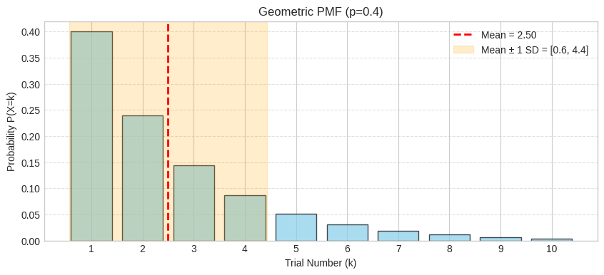
Let’s visualize a Geometric distribution with $p = 0.4$ (our free throw example):

# Remove existing SVG if present
if os.path.exists('ch07_geometric_pmf_generic.svg'):
    os.remove('ch07_geometric_pmf_generic.svg')

# Create Geometric distribution for visualization (p=0.4)
p_viz = 0.4
geom_viz = stats.geom(p=p_viz)

# Calculate mean and std (adjusted for trial number definition)
mean_viz = 1 / p_viz
std_viz = np.sqrt((1 - p_viz) / p_viz**2)

# Plotting the PMF
k_values_viz = np.arange(1, 11)
pmf_values_viz = geom_viz.pmf(k_values_viz)

plt.figure(figsize=(10, 4))
plt.bar(k_values_viz, pmf_values_viz, color='skyblue', edgecolor='black', alpha=0.7)

# Add mean line
plt.axvline(mean_viz, color='red', linestyle='--', linewidth=2, label=f'Mean = {mean_viz:.2f}')

# Add mean ± 1 std region
plt.axvspan(mean_viz - std_viz, mean_viz + std_viz, alpha=0.2, color='orange',
            label=f'Mean ± 1 SD = [{mean_viz - std_viz:.1f}, {mean_viz + std_viz:.1f}]')

plt.title(f"Geometric PMF (p={p_viz})")
plt.xlabel("Trial Number (k)")
plt.ylabel("Probability P(X=k)")
plt.xticks(k_values_viz)
plt.legend(loc='upper right', fontsize=10)
plt.grid(axis='y', linestyle='--', alpha=0.6)
plt.savefig('ch07_geometric_pmf_generic.svg', format='svg', bbox_inches='tight')
plt.show()

The PMF shows exponentially decreasing probabilities - you’re most likely to succeed on the first few trials. The shaded region shows mean ± 1 standard deviation.

# Remove existing SVG if present
if os.path.exists('ch07_geometric_cdf_generic.svg'):
    os.remove('ch07_geometric_cdf_generic.svg')

# Plotting the CDF
cdf_values_viz = geom_viz.cdf(k_values_viz)

plt.figure(figsize=(10, 4))
plt.step(k_values_viz, cdf_values_viz, where='post', color='darkgreen', linewidth=2)

# Add mean line
plt.axvline(mean_viz, color='red', linestyle='--', linewidth=2, label=f'Mean = {mean_viz:.2f}')

plt.title(f"Geometric CDF (p={p_viz})")
plt.xlabel("Trial Number (k)")
plt.ylabel("Cumulative Probability P(X <= k)")
plt.xticks(k_values_viz)
plt.legend(loc='lower right', fontsize=10)
plt.grid(True, which='both', linestyle='--', linewidth=0.5, alpha=0.6)
plt.savefig('ch07_geometric_cdf_generic.svg', format='svg', bbox_inches='tight')
plt.show()

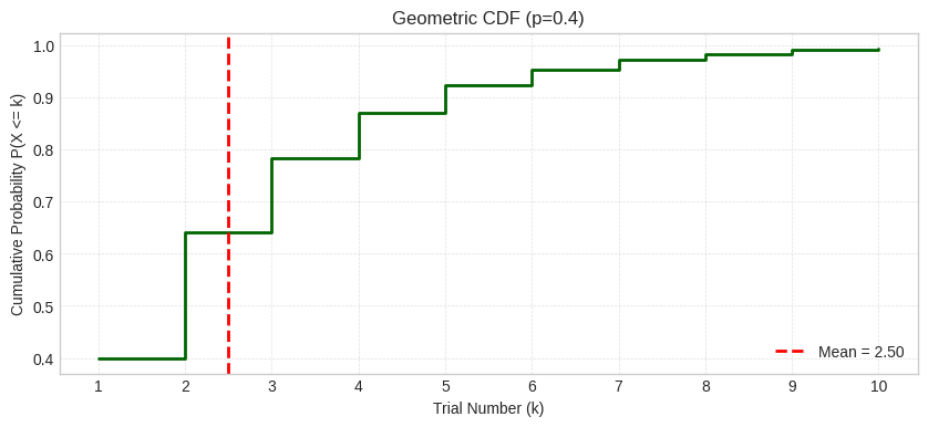
The CDF shows P(X ≤ k), approaching 1 as k increases (eventually you’ll succeed). The red dashed line marks the mean.

Example: Certification Exam with p = 0.6

Modeling the number of attempts needed to pass a certification exam where the pass probability is 0.6.

Let’s use scipy.stats.geom to explore probabilities and compute expected values. Remember that scipy’s definition counts failures before the first success, so we’ll translate between the two interpretations.

Setting up the distribution:

We create a geometric distribution with a success probability of 0.6 (60% pass rate):

import numpy as np
from scipy import stats
import matplotlib.pyplot as plt

# Using scipy.stats.geom
p_pass = 0.6
geom_rv = stats.geom(p=p_pass)

Calculating specific probabilities using the PMF:

What’s the probability of passing for the first time on the 3rd attempt? This means failing the first two attempts and passing on the third:

# PMF: Probability that the first success occurs on trial k (k=1, 2, ...)
k_trial = 3 # Third attempt
print(f"P(First pass on attempt {k_trial}): {geom_rv.pmf(k_trial):.4f}")

P(First pass on attempt 3): 0.0960

There’s a 9.6% chance of passing on exactly the 3rd attempt. This is calculated as (1-0.6)² × 0.6 = 0.4² × 0.6 = 0.096.

Calculating cumulative probabilities using the CDF:

What’s the probability of passing within the first 2 attempts?

# CDF: Probability that the first success occurs on or before trial k
k_or_before = 2
print(f"P(First pass on or before attempt {k_or_before}): {geom_rv.cdf(k_or_before):.4f}")
print(f"P(First pass takes more than {k_or_before} attempts): {1 - geom_rv.cdf(k_or_before):.4f}")
print(f"P(First pass takes more than {k_or_before} attempts) (using sf): {geom_rv.sf(k_or_before):.4f}")

P(First pass on or before attempt 2): 0.8400
P(First pass takes more than 2 attempts): 0.1600
P(First pass takes more than 2 attempts) (using sf): 0.1600

There’s an 84% chance of passing within 2 attempts, meaning only a 16% chance you’ll need more than 2 attempts.

Computing mean and variance:

Let’s find the expected number of attempts needed:

# Mean and Variance
mean_trials = geom_rv.mean()
var_trials = geom_rv.var()
print(f"Mean number of attempts until first pass: {mean_trials:.2f}")
print(f"Variance of number of attempts: {var_trials:.2f}")

Mean number of attempts until first pass: 1.67
Variance of number of attempts: 1.11

On average, you expect to need 1.67 attempts (which matches the formula 1/p = 1/0.6). The relatively low variance suggests most people will pass within the first few attempts.

Generating random samples:

We can simulate many students taking the exam repeatedly until they pass:

# Generate random samples (trial numbers until first success)
n_simulations = 1000
samples_trials = geom_rv.rvs(size=n_simulations)
# print(f"\nSimulated number of attempts until first pass ({n_simulations} simulations): {samples_trials[:20]}...")

These 1000 samples show the natural variation in how many attempts different students might need.

Visualizing the PMF:

Let’s visualize the probability of passing on each attempt number (showing the first 10 attempts):

# Plotting the PMF (using trial number k=1, 2, ...)
k_values_trials = np.arange(1, 11) # Plot first 10 trials
pmf_values = geom_rv.pmf(k_values_trials)

plt.figure(figsize=(8, 3.5))
plt.bar(k_values_trials, pmf_values, color='skyblue', edgecolor='black', alpha=0.7)
plt.title(f"Geometric PMF (p={p_pass})")
plt.xlabel("Trial Number (k)")
plt.ylabel("Probability P(X=k)")
plt.xticks(k_values_trials)
plt.grid(axis='y', linestyle='--', alpha=0.6)
plt.show()

The PMF shows exponentially decreasing probabilities - you’re most likely to pass on the first attempt (60%), then second attempt (24%), and so on. This characteristic “memoryless” exponential decay is unique to the geometric distribution. Notice how the bars get progressively smaller, with very low probabilities by attempt 5 or 6.

Visualizing the CDF:

The cumulative distribution shows the probability of passing by a given attempt:

# Plotting the CDF (using trial number k=1, 2, ...)
cdf_values = geom_rv.cdf(k_values_trials)

plt.figure(figsize=(8, 3.5))
plt.step(k_values_trials, cdf_values, where='post', color='darkgreen', linewidth=2)
plt.title(f"Geometric CDF (p={p_pass})")
plt.xlabel("Trial Number (k)")
plt.ylabel("Cumulative Probability P(X <= k)")
plt.xticks(k_values_trials)
plt.grid(True, which='both', linestyle='--', linewidth=0.5, alpha=0.6)
plt.show()

The CDF shows P(X ≤ k), rapidly approaching 1 as the attempt number increases. By attempt 2, there’s an 84% chance of having passed, and by attempt 5, it’s over 99%. This confirms that with p = 0.6, most people will pass within the first few attempts.

Quick Check Questions

You flip a coin until you get your first Heads. What distribution models this and what is the parameter?

Answer

Geometric distribution with p = 0.5 - Counting trials until first success, each trial has p = 0.5 success probability.

For a Geometric distribution with p = 0.25, what is the expected value (mean)?

Answer

E[X] = 1/p = 1/0.25 = 4 - Expected number of trials until first success.

You’re calling customer service and have a 20% chance each attempt of getting through. Should you model this with Geometric or Binomial?

Answer

Geometric distribution - You’re waiting for the first success (getting through), not counting successes in a fixed number of tries. Geometric models “how many attempts until success” with p = 0.20.

Binomial would apply if you made a fixed number of calls and counted how many got through.

Which is more likely for a Geometric distribution with p = 0.5: success on the 1st trial or success on the 3rd trial?

Answer

1st trial is more likely - The Geometric PMF decreases exponentially with k, so P(X=1) > P(X=3).

Specifically: P(X=1) = 0.5, while P(X=3) = (0.5)³ = 0.125

For a Geometric distribution, why does the variance equal (1-p)/p²?

Answer

The variance formula Var(X) = (1-p)/p² reflects the increasing uncertainty as p decreases:

When p is high (easy to succeed): variance is low (more predictable)
When p is low (hard to succeed): variance is high (could take many tries or get lucky early)

For example:

p = 0.5: Var(X) = 0.5/0.25 = 2
p = 0.1: Var(X) = 0.9/0.01 = 90 (much more variable!)

4. Negative Binomial Distribution¶

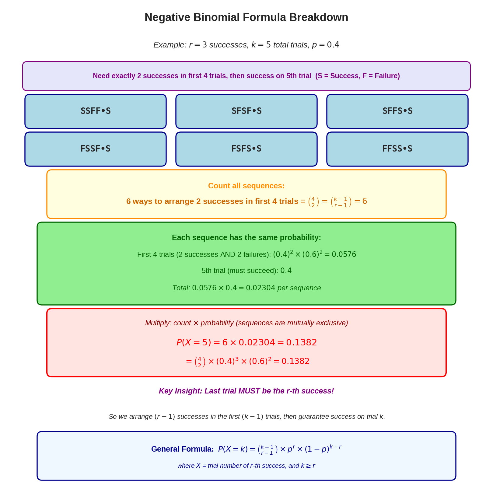
The Negative Binomial distribution models the number of independent Bernoulli trials needed to achieve a fixed number of successes ( $r$ ). It generalizes the Geometric distribution (where $r=1$ ).

Concrete Example

You’re rolling a die until you get 3 sixes. Each roll has p = 1/6 probability of rolling a six. How many rolls will it take to get your 3rd six?

We model this with a random variable $X$ :

$X$ = the trial number on which the 3rd six appears
$X$ can take values 3, 4, 5, ... (minimum 3 rolls, could be more)

The probabilities are:

$P(X = 3)$ = all three rolls are sixes
$P(X = 4)$ = 2 sixes in first 3 rolls, then a six on 4th roll
And so on...

The Negative Binomial PMF

For trials with success probability $p$ and target $r$ successes:

P(X=k) = \binom{k-1}{r-1} p^r (1-p)^{k-r}

(9)

for $k = r, r+1, r+2, \dots$

Understanding the formula: This means $r-1$ successes in the first $k-1$ trials, and the $k$ -th trial is the $r$ -th success.

Why This Formula Works

To build intuition, let’s see how the formula breaks down into three parts:

$\binom{k-1}{r-1}$ : Choose which $r-1$ of the first $k-1$ trials are successes (the $k$ -th trial must be a success, so we only choose positions for $r-1$ successes)
$p^r$ : Probability of $r$ successes
$(1-p)^{k-r}$ : Probability of $k-r$ failures

Intuitive example: For $r=3$ successes in $k=5$ trials with $p=0.4$ :

Need exactly 2 successes in first 4 trials: $\binom{4}{2} = 6$ ways (e.g., SSFF, SFSF, SFFS, FSSF, FSFS, FFSS)
Each arrangement has probability $(0.4)^2 (0.6)^2$ for the first 4 trials
5th trial must succeed: 0.4
Combined: $P(X=5) = \binom{4}{2} \times (0.4)^3 \times (0.6)^2 = 6 \times (0.4)^3 \times (0.6)^2 = 0.2304$

This demonstrates how the formula $P(X=k) = \binom{k-1}{r-1} p^r (1-p)^{k-r}$ combines all three parts.

The binomial coefficient ensures we count all possible arrangements where the $r$ -th success occurs exactly on trial $k$ . (We’ll see this visually in the diagram below.)

Now let’s mechanically apply the formula to our die example with different parameters: For $P(X=4)$ (the probability it takes exactly 4 rolls to get the 3rd six) with $r=3$ sixes and $p=1/6$ :

Substituting $k=4$ , $r=3$ , $p=1/6$ into the formula:

\begin{align} P(X=k) &= \binom{k-1}{r-1} p^r (1-p)^{k-r} \\ P(X=4) &= \binom{4-1}{3-1}(1/6)^3(5/6)^{4-3} \\ &= \binom{3}{2}(1/6)^3(5/6)^1 \\ &= 3 \times \frac{1}{216} \times \frac{5}{6} \\ &= \frac{15}{1296} \\ &\approx 0.0116 \end{align}

(10)

Visual breakdown: The following diagram shows how the negative binomial formula counts all possible sequences and combines their probabilities:

# Remove existing SVG if present
if os.path.exists('ch07_negative_binomial_formula_breakdown.svg'):
    os.remove('ch07_negative_binomial_formula_breakdown.svg')

import matplotlib.pyplot as plt
import matplotlib.patches as mpatches

# --- Settings ---
BOX_PAD = 0.01  # single, consistent pad for every rounded box (fixes uneven visible gaps)

# Create figure for formula breakdown
fig, ax = plt.subplots(figsize=(16, 16))

# Make axes fill the whole figure so "axes coords" behave predictably
fig.subplots_adjust(left=0, right=1, top=1, bottom=0)

ax.set_xlim(0, 1)
ax.set_ylim(0, 1)
ax.axis('off')

# Define all CONTENT heights (actual elements)
title_height = 0.03
subtitle_height = 0.025
param_box_height = 0.04
seq_box_height = 0.05
count_box_height = 0.08
prob_box_height = 0.15
result_box_height = 0.12
key_insight_text_height = 0.025
key_explain_text_height = 0.025
formula_box_height = 0.08

# Calculate total content height
total_content_height = (
    title_height +
    subtitle_height +
    param_box_height +
    seq_box_height * 2 +  # Two rows of sequence boxes
    count_box_height +
    prob_box_height +
    result_box_height +
    key_insight_text_height +
    key_explain_text_height +
    formula_box_height
)

# Calculate available space for gaps
top_margin = 0.02
bottom_margin = 0.03
usable_height = 1.0 - top_margin - bottom_margin
whitespace = usable_height - total_content_height

# Number of gaps between sections
num_gaps = 10

# Calculate uniform gap size
gap = whitespace / num_gaps

def add_box(x, y, w, h, edge, face, lw, z=1):
    """Consistent rounded box with a single pad value."""
    patch = mpatches.FancyBboxPatch(
        (x, y), w, h,
        boxstyle=f"round,pad={BOX_PAD}",
        linewidth=lw,
        edgecolor=edge,
        facecolor=face,
        zorder=z
    )
    ax.add_patch(patch)
    return patch

# Build layout from top down with calculated gaps
current_y = 1.0 - top_margin

# Title
ax.text(0.5, current_y, "Negative Binomial Formula Breakdown",
        transform=ax.transAxes, ha="center", va="top",
        fontsize=26, weight="bold")
current_y -= title_height + gap

# Subtitle
ax.text(0.5, current_y, r"Example: $r=3$ successes, $k=5$ total trials, $p=0.4$",
        transform=ax.transAxes, ha="center", va="top",
        fontsize=19, style="italic")
current_y -= subtitle_height + gap

# Parameters box
param_box_bottom = current_y - param_box_height
add_box(0.05, param_box_bottom, 0.90, param_box_height,
        edge='purple', face='lavender', lw=2, z=1)
ax.text(0.5, param_box_bottom + param_box_height/2,
        "Need exactly 2 successes in first 4 trials, then success on 5th trial  (S = Success, F = Failure)",
        transform=ax.transAxes, ha="center", va="center",
        fontsize=16.5, weight="bold", color="purple")
current_y = param_box_bottom - gap

# Sequence boxes - First row
sequences = ["SSFF•S", "SFSF•S", "SFFS•S", "FSSF•S", "FSFS•S", "FFSS•S"]
seq_row1_bottom = current_y - seq_box_height
for i in range(3):
    x_pos = 0.055 + i * 0.31
    add_box(x_pos, seq_row1_bottom, 0.27, seq_box_height,
            edge='darkblue', face='lightblue', lw=2.5, z=2)
    ax.text(x_pos + 0.135, seq_row1_bottom + seq_box_height/2, sequences[i],
            transform=ax.transAxes, ha="center", va="center",
            fontsize=20, weight="bold", family='monospace', zorder=3)

# Sequence boxes - Second row
current_y = seq_row1_bottom - gap
seq_row2_bottom = current_y - seq_box_height
for i in range(3):
    x_pos = 0.055 + i * 0.31
    add_box(x_pos, seq_row2_bottom, 0.27, seq_box_height,
            edge='darkblue', face='lightblue', lw=2.5, z=2)
    ax.text(x_pos + 0.135, seq_row2_bottom + seq_box_height/2, sequences[i+3],
            transform=ax.transAxes, ha="center", va="center",
            fontsize=20, weight="bold", family='monospace', zorder=3)
current_y = seq_row2_bottom - gap

# Counting explanation box
count_box_bottom = current_y - count_box_height
add_box(0.10, count_box_bottom, 0.80, count_box_height,
        edge='darkorange', face='lightyellow', lw=2.5, z=1)
ax.text(0.5, count_box_bottom + count_box_height * 0.70, r"Count all sequences:",
        transform=ax.transAxes, ha="center", va="center",
        fontsize=18, weight="bold", color='darkorange', zorder=4)
ax.text(0.5, count_box_bottom + count_box_height * 0.30,
        r"6 ways to arrange 2 successes in first 4 trials = $\binom{4}{2} = \binom{k-1}{r-1} = 6$",
        transform=ax.transAxes, ha="center", va="center",
        fontsize=19, weight="bold", color='#CC6600', zorder=4)
current_y = count_box_bottom - gap

# Probability calculation box
prob_box_bottom = current_y - prob_box_height
add_box(0.08, prob_box_bottom, 0.84, prob_box_height,
        edge='darkgreen', face='lightgreen', lw=2.5, z=1)
ax.text(0.5, prob_box_bottom + prob_box_height * 0.85,
        "Each sequence has the same probability:",
        transform=ax.transAxes, ha="center", va="center",
        fontsize=18, weight="bold", color='darkgreen', zorder=4)
ax.text(0.5, prob_box_bottom + prob_box_height * 0.62,
        r"First 4 trials (2 successes AND 2 failures): $(0.4)^2 \times (0.6)^2 = 0.0576$",
        transform=ax.transAxes, ha="center", va="center",
        fontsize=17, color='darkgreen', zorder=4)
ax.text(0.5, prob_box_bottom + prob_box_height * 0.40,
        r"5th trial (must succeed): $0.4$",
        transform=ax.transAxes, ha="center", va="center",
        fontsize=17, color='darkgreen', zorder=4)
ax.text(0.5, prob_box_bottom + prob_box_height * 0.16,
        r"Total: $0.0576 \times 0.4 = 0.02304$ per sequence",
        transform=ax.transAxes, ha="center", va="center",
        fontsize=17, style="italic", color='darkgreen', zorder=4)
current_y = prob_box_bottom - gap

# Final result box
result_box_bottom = current_y - result_box_height
add_box(0.10, result_box_bottom, 0.80, result_box_height,
        edge='red', face='mistyrose', lw=3, z=1)
ax.text(0.5, result_box_bottom + result_box_height * 0.83,
        r"Multiply: count $\times$ probability (sequences are mutually exclusive)",
        transform=ax.transAxes, ha="center", va="center",
        fontsize=17, style="italic", color='darkred', zorder=4)
ax.text(0.5, result_box_bottom + result_box_height * 0.50,
        r"$P(X=5) = 6 \times 0.02304 = 0.1382$",
        transform=ax.transAxes, ha="center", va="center",
        fontsize=21, weight="bold", color='red', zorder=4)
ax.text(0.5, result_box_bottom + result_box_height * 0.17,
        r"$= \binom{4}{2} \times (0.4)^3 \times (0.6)^2 = 0.1382$",
        transform=ax.transAxes, ha="center", va="center",
        fontsize=19, color='red', zorder=4)
current_y = result_box_bottom - gap

# Key insight text
key_insight_y = current_y - key_insight_text_height/2
ax.text(0.5, key_insight_y,
        "Key Insight: Last trial MUST be the r-th success!",
        transform=ax.transAxes, ha="center", va="center",
        fontsize=18, style="italic", weight="bold", color='purple', zorder=4)
current_y -= key_insight_text_height + gap

# Explanation text
key_explain_y = current_y - key_explain_text_height/2
ax.text(0.5, key_explain_y,
        r"So we arrange $(r-1)$ successes in the first $(k-1)$ trials, then guarantee success on trial $k$.",
        transform=ax.transAxes, ha="center", va="center",
        fontsize=16, style="italic", zorder=4)
current_y -= key_explain_text_height + gap

# General formula box
formula_box_bottom = current_y - formula_box_height
add_box(0.08, formula_box_bottom, 0.84, formula_box_height,
        edge='darkblue', face='aliceblue', lw=2.5, z=1)
ax.text(0.5, formula_box_bottom + formula_box_height * 0.65,
        r"General Formula:  $P(X = k) = \binom{k-1}{r-1} \times p^r \times (1-p)^{k-r}$",
        transform=ax.transAxes, ha="center", va="center",
        fontsize=18, weight="bold", color='darkblue', zorder=4)
ax.text(0.5, formula_box_bottom + formula_box_height * 0.25,
        r"where $X$ = trial number of $r$-th success, and $k \geq r$",
        transform=ax.transAxes, ha="center", va="center",
        fontsize=15, style="italic", color='darkblue', zorder=4)

plt.savefig('ch07_negative_binomial_formula_breakdown.svg', format='svg', bbox_inches='tight', pad_inches=0.25)
plt.show()

The diagram shows how the negative binomial formula works: we need exactly $r-1$ successes in the first $k-1$ trials (which can be arranged in $\binom{k-1}{r-1}$ ways), and then the $k$ -th trial must be a success. Each of the 6 sequences shown has the same probability, and we multiply by the number of sequences to get the total probability.

Now that we understand the formula and its visualization, let’s summarize the essential properties of the negative binomial distribution:

Key Characteristics

Scenarios: Coin flips until getting r Heads, products inspected to find r defects, interviews until making r hires
Parameters:
- $r$ : target number of successes ( $r \ge 1$ )
- $p$ : probability of success on each trial ( $0 < p \le 1$ )
Random Variable: $X \in \{r, r+1, r+2, ...\}$

Mean: $E[X] = \frac{r}{p}$

Variance: $Var(X) = \frac{r(1-p)}{p^2}$

Standard Deviation: $SD(X) = \frac{\sqrt{r(1-p)}}{p}$

Visualizing the Distribution

Let’s visualize our die example: Negative Binomial distribution with $r = 3$ sixes and $p = 1/6$ :

# Remove existing SVG if present
if os.path.exists('ch07_negative_binomial_pmf_generic.svg'):
    os.remove('ch07_negative_binomial_pmf_generic.svg')

# Create Negative Binomial distribution for our die example (r=3, p=1/6)
r_viz = 3
p_viz = 1/6
nbinom_viz = stats.nbinom(n=r_viz, p=p_viz)

# Calculate mean and std
mean_viz = r_viz / p_viz
std_viz = np.sqrt(r_viz * (1 - p_viz)) / p_viz

# Plotting the PMF
k_values_viz = np.arange(r_viz, 45)  # Total trials from r to 45 (wider range for p=1/6)
pmf_values_viz = nbinom_viz.pmf(k_values_viz - r_viz)  # Adjust for scipy

plt.figure(figsize=(10, 4))
plt.bar(k_values_viz, pmf_values_viz, color='skyblue', edgecolor='black', alpha=0.7)

# Add mean line
plt.axvline(mean_viz, color='red', linestyle='--', linewidth=2, label=f'Mean = {mean_viz:.1f}')

# Add mean ± 1 std region
plt.axvspan(mean_viz - std_viz, mean_viz + std_viz, alpha=0.2, color='orange',
            label=f'Mean ± 1 SD = [{mean_viz - std_viz:.1f}, {mean_viz + std_viz:.1f}]')

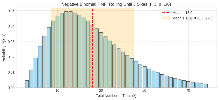
plt.title(f"Negative Binomial PMF: Rolling Until 3 Sixes (r={r_viz}, p=1/6)")
plt.xlabel("Total Number of Trials (k)")
plt.ylabel("Probability P(X=k)")
plt.legend(loc='upper right', fontsize=10)
plt.grid(axis='y', linestyle='--', alpha=0.6)
plt.savefig('ch07_negative_binomial_pmf_generic.svg', format='svg', bbox_inches='tight')
plt.show()

The PMF shows the distribution is centered around the expected value r/p = 3/(1/6) = 18 trials. You can see our calculated P(X=4) ≈ 0.0116 as a small bar near the left tail at k=4. The shaded region shows mean ± 1 standard deviation.

# Remove existing SVG if present
if os.path.exists('ch07_negative_binomial_cdf_generic.svg'):
    os.remove('ch07_negative_binomial_cdf_generic.svg')

# Plotting the CDF
cdf_values_viz = nbinom_viz.cdf(k_values_viz - r_viz)

plt.figure(figsize=(10, 4))
plt.step(k_values_viz, cdf_values_viz, where='post', color='darkgreen', linewidth=2)

# Add mean line
plt.axvline(mean_viz, color='red', linestyle='--', linewidth=2, label=f'Mean = {mean_viz:.1f}')

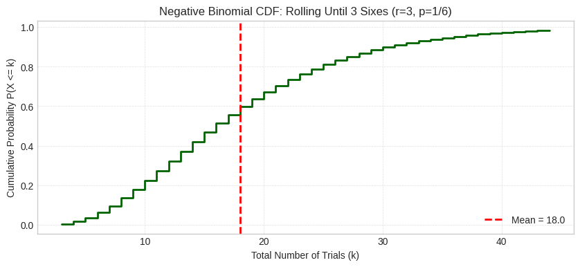
plt.title(f"Negative Binomial CDF: Rolling Until 3 Sixes (r={r_viz}, p=1/6)")
plt.xlabel("Total Number of Trials (k)")
plt.ylabel("Cumulative Probability P(X <= k)")
plt.legend(loc='lower right', fontsize=10)
plt.grid(True, which='both', linestyle='--', linewidth=0.5, alpha=0.6)
plt.savefig('ch07_negative_binomial_cdf_generic.svg', format='svg', bbox_inches='tight')
plt.show()

The CDF shows P(X ≤ k), the cumulative probability of getting 3 sixes within k rolls. At k=4, the CDF shows P(X ≤ 4) = P(X=3) + P(X=4) ≈ 0.0046 + 0.0116 ≈ 0.0162, which is the very low cumulative probability in the left tail. The red dashed line marks the mean (18 trials).

Example: Quality Control with r = 3, p = 0.05

A quality control inspector tests electronic components until finding 3 defective ones. The defect rate is p = 0.05.

We’ll use scipy.stats.nbinom to calculate the probability of needing a certain number of trials and compute expected values, keeping in mind scipy’s definition of counting failures.

Setting up the distribution:

First, we create the negative binomial distribution object with our parameters:

import numpy as np
from scipy import stats
import matplotlib.pyplot as plt

# Using scipy.stats.nbinom
r_defective = 3
p_defective = 0.05
nbinom_rv = stats.nbinom(n=r_defective, p=p_defective)

Calculating specific probabilities using the PMF:

What’s the probability we need to test exactly 80 components to find 3 defective ones? Remember that scipy counts failures (good components), so we need to convert:

# PMF: Probability of needing k components tested to find r defective
k_components = 80
num_good = k_components - r_defective
if num_good >= 0:
    prob_k_components = nbinom_rv.pmf(num_good)
    print(f"P(Need exactly {k_components} components to find {r_defective} defective): {prob_k_components:.4f}")
else:
    print(f"Cannot find {r_defective} defective in fewer than {r_defective} components.")

P(Need exactly 80 components to find 3 defective): 0.0074

This probability is quite low (0.0074 or 0.74%) because 80 components is far from the expected value.

Calculating cumulative probabilities using the CDF:

What if we want to know the probability of finding 3 defective components within 100 tests?

# CDF: Probability of needing k or fewer components
k_or_fewer_components = 100
num_good_max = k_or_fewer_components - r_defective
if num_good_max >= 0:
    prob_k_or_fewer = nbinom_rv.cdf(num_good_max)
    print(f"P(Need {k_or_fewer_components} or fewer components to find {r_defective} defective): {prob_k_or_fewer:.4f}")
else:
    print(f"Cannot find {r_defective} defective in fewer than {r_defective} components.")

P(Need 100 or fewer components to find 3 defective): 0.8817

There’s an 88.17% chance we’ll find all 3 defective components within the first 100 tests. This makes sense because 100 is well above the expected value (as we’ll see below).

Understanding scipy’s parameterization:

Scipy’s nbinom counts the number of non-defective (good) components before finding r defective ones. This is subtly different from counting total components tested:

# Mean and Variance (scipy's definition: number of non-defective items)
mean_good_scipy = nbinom_rv.mean()
var_good_scipy = nbinom_rv.var()
print(f"Mean number of good components before {r_defective} defective (scipy): {mean_good_scipy:.2f}")
print(f"Variance of good components before {r_defective} defective (scipy): {var_good_scipy:.2f}")

Mean number of good components before 3 defective (scipy): 57.00
Variance of good components before 3 defective (scipy): 1140.00

Scipy tells us we expect to see 57 good components before finding 3 defective ones.

Converting to total components (our interpretation):

For practical purposes, we often care about the total number of components we need to test (good + defective). We can calculate this directly using our formulas $E[X] = r/p$ and $Var(X) = r(1-p)/p^2$ :

# Mean and Variance (our definition: total components tested)
mean_components = r_defective / p_defective
var_components = r_defective * (1 - p_defective) / p_defective**2
print(f"Mean number of components to test for {r_defective} defective: {mean_components:.2f}")
print(f"Variance of number of components: {var_components:.2f}")

Mean number of components to test for 3 defective: 60.00
Variance of number of components: 1140.00

On average, we expect to test 60 components total to find 3 defective ones (57 good + 3 defective). Note that the variance is the same (1140) in both parameterizations—we’re just shifting the distribution by adding the constant r = 3.

Generating random samples:

We can simulate the inspection process by generating random samples. Each sample represents one complete “run” of testing components until we find 3 defective ones:

# Generate random samples (number of good components before r defective)
n_simulations = 1000
samples_good_nb = nbinom_rv.rvs(size=n_simulations)
# Convert to total components tested (good + r defective)
samples_components_nb = samples_good_nb + r_defective
# print(f"\nSimulated components tested to find {r_defective} defective ({n_simulations} sims): {samples_components_nb[:20]}...")

These samples could be used for Monte Carlo simulation or to verify our theoretical calculations.

Visualizing the PMF:

Let’s visualize the full probability distribution to see the range of likely outcomes:

# Plotting the PMF (using total components tested k = r, r+1, ...)
k_values_components = np.arange(r_defective, r_defective + 150) # Plot a range
pmf_values_nb = nbinom_rv.pmf(k_values_components - r_defective) # Adjust k for scipy

plt.figure(figsize=(8, 3.5))
plt.bar(k_values_components, pmf_values_nb, color='skyblue', edgecolor='black', alpha=0.7)
plt.title(f"Negative Binomial PMF (r={r_defective}, p={p_defective})")
plt.xlabel("Total Number of Components Tested (k)")
plt.ylabel("Probability P(X=k)")
plt.grid(axis='y', linestyle='--', alpha=0.6)
plt.show()

The PMF shows the distribution centered around r/p = 60 components with considerable variability. The distribution is right-skewed, meaning there’s a long tail of possibilities where we might need many more components than average. Notice how the probability at k=80 (which we calculated earlier as 0.0074) appears as a small bar in the right tail.

Visualizing the CDF:

The cumulative distribution function helps us answer questions like “What’s the probability we’ll be done within k tests?”

# Plotting the CDF (using total components tested k = r, r+1, ...)
cdf_values_nb = nbinom_rv.cdf(k_values_components - r_defective) # Adjust k for scipy

plt.figure(figsize=(8, 3.5))
plt.step(k_values_components, cdf_values_nb, where='post', color='darkgreen', linewidth=2)
plt.title(f"Negative Binomial CDF (r={r_defective}, p={p_defective})")
plt.xlabel("Total Number of Components Tested (k)")
plt.ylabel("Cumulative Probability P(X <= k)")
plt.grid(True, which='both', linestyle='--', linewidth=0.5, alpha=0.6)
plt.show()

The CDF shows P(X ≤ k), the cumulative probability of finding 3 defective items within k tests. The S-curve shape is characteristic of CDFs. We can see that by k=100 tests, the CDF reaches approximately 0.88 (matching our earlier calculation of 88.17%). The CDF crosses 0.5 around k=53, meaning there’s a 50% chance we’ll need 53 or fewer tests to find all 3 defective components.

Quick Check Questions

You flip a fair coin until you get 5 Heads. What distribution models this and what are the parameters?

Answer

Negative Binomial with r = 5, p = 0.5 - Counting trials until getting r successes, each trial has p = 0.5.

For a Negative Binomial distribution with r = 4 and p = 0.5, what is the expected value (mean)?

Answer

E[X] = r/p = 4/0.5 = 8 - Expected number of trials to get 4 successes.

A basketball player practices free throws until making 10 successful shots. Each shot has a 70% success rate. Which distribution and why?

Answer

Negative Binomial with r = 10, p = 0.7 - We’re waiting for a fixed number of successes (r = 10), not just the first success. Each trial (shot) is independent with constant probability p = 0.7.

This is NOT Geometric because we need 10 successes, not just 1.

How is Negative Binomial related to Geometric distribution?

Answer

Geometric is a special case where r = 1 - Negative Binomial with r=1 is identical to Geometric.

Geometric: waiting for 1st success
Negative Binomial: waiting for r-th success (r ≥ 1)

For Negative Binomial, why is the variance r(1-p)/p²?

Answer

The variance r(1-p)/p² grows with both r and uncertainty:

Increases with r: Waiting for more successes means more trials and more variability
Increases as p decreases: Lower success probability means higher uncertainty in when you’ll reach r successes

For example:

r=1, p=0.5: Var = 1×0.5/0.25 = 2
r=5, p=0.5: Var = 5×0.5/0.25 = 10 (more variable with more successes needed)
r=5, p=0.2: Var = 5×0.8/0.04 = 100 (much more variable with low p!)

5. Poisson Distribution¶

The Poisson distribution models the number of events occurring in a fixed interval of time or space when events happen independently at a constant average rate.

Concrete Example

You receive an average of 4 customer calls per hour. How many calls will you get in the next hour?

We model this with a random variable $X$ :

$X$ = the number of calls in one hour
$X$ can take values 0, 1, 2, 3, ... (any non-negative integer)

The average rate is $\lambda = 4$ calls/hour.

The Poisson PMF

For events occurring at average rate $\lambda$ :

P(X=k) = \frac{e^{-\lambda} \lambda^k}{k!} \quad \text{for } k = 0, 1, 2, \dots

(11)

where $e \approx 2.71828$ is Euler’s number.

Let’s verify for our example (λ=4):

$P(X=4) = \frac{e^{-4} \times 4^4}{4!} \approx 0.195$ ✓

Why This Formula Works

The Poisson formula $\frac{e^{-\lambda} \lambda^k}{k!}$ emerges from the mathematics of rare events:

$\lambda^k / k!$ : Represents the “raw” likelihood of $k$ events based on the rate $\lambda$
$e^{-\lambda}$ : A normalization factor that ensures all probabilities sum to 1

Intuition: The Poisson distribution arises as the limit of the Binomial distribution when:

You divide a time interval into many tiny sub-intervals ( $n$ very large)
The probability of an event in each sub-interval is very small ( $p$ very small)
The average rate $\lambda = np$ stays constant

For example, “4 calls per hour” could be modeled as 3600 one-second intervals where each second has probability $p = 4/3600$ of receiving a call.

Why mean = variance = λ? This unique property reflects the “memoryless” nature of the Poisson process - events occur randomly and independently at a constant average rate.

Algorithm visualization: The following diagram visualizes the Poisson formula as competing forces, building intuition for why each component exists:

import matplotlib.pyplot as plt
import numpy as np
from scipy.stats import poisson
from scipy.special import factorial
import matplotlib.patches as mpatches

def create_poisson_visual(lam=4):
    """Poisson distribution visualization showing the 'forces' intuition"""
    k_max = 9
    k_vals = np.arange(k_max + 1)

    # Calculate components - the three "forces"
    numerator = np.power(lam, k_vals)  # Driver
    denominator = factorial(k_vals)     # Brake
    constant = np.exp(-lam)             # Scaler
    prob = poisson.pmf(k_vals, lam)

    # Setup figure - optimized for mobile viewing
    fig, ax = plt.subplots(figsize=(14, 9))
    ax.axis('off')
    ax.set_xlim(-0.5, 11.5)
    ax.set_ylim(0, 10)

    # Layout constants - narrower boxes
    box_width = 0.95
    box_height = 0.9
    gap = 0.2
    start_y = 6.5

    # Title
    ax.text((k_max * (box_width + gap))/2, 9.5,
            f'Visualizing Poisson: The Three Forces ($\lambda = {lam}$)',
            ha='center', fontsize=22, fontweight='bold', color='#333333')

    ax.text((k_max * (box_width + gap))/2, 9.0,
            f'Expected rate: {lam} events. Probability of exactly k events?',
            ha='center', fontsize=15, color='#555555')

    # Draw probability boxes for each k value
    for i, k in enumerate(k_vals):
        x = i * (box_width + gap)

        # Color intensity based on probability
        max_p = max(prob)
        alpha = 0.1 + 0.8 * (prob[i] / max_p)
        box_color = plt.cm.Blues(alpha)

        # Rounded rectangle for each k
        rect = mpatches.FancyBboxPatch((x, start_y), box_width, box_height,
                                   boxstyle="round,pad=0.1",
                                   facecolor=box_color, edgecolor='#2c3e50', linewidth=1.5)
        ax.add_patch(rect)

        # k label
        center_x = x + box_width/2
        center_y = start_y + box_height/2
        ax.text(center_x, center_y, f'k={k}',
                ha='center', va='center', fontsize=17, fontweight='bold',
                color='black' if alpha < 0.6 else 'white')

        # Formula and result below box - larger fonts, better spacing
        calc_text = f"$\\frac{{{lam}^{{{k}}} \\cdot e^{{-{lam}}}}}{{{int(denominator[i])}}}$"
        result_text = f"= {prob[i]:.4f}"

        ax.text(center_x, start_y - 0.35, calc_text,
                ha='center', va='top', fontsize=15, color='#333333')
        ax.text(center_x, start_y - 1.05, result_text,
                ha='center', va='top', fontsize=13, fontweight='bold', color='#333333')

    # The Three Forces - Explanatory boxes with better positioning

    # Force 1: The Driver (Numerator)
    bbox_driver = dict(boxstyle="round,pad=0.5", fc="#fae5d3", ec="#d35400", lw=1.5)
    ax.text(1.2, 3.3, "Force 1: The Driver\n(Numerator)\n\n" + r"$\lambda^k$" +
            "\n\nPushes UP exponentially.\nHigher λ or k → more likely.",
            ha='center', va='top', fontsize=12, bbox=bbox_driver, color='#873600')

    # Force 2: The Brake (Denominator)
    bbox_brake = dict(boxstyle="round,pad=0.5", fc="#d5f5e3", ec="#27ae60", lw=1.5)
    ax.text(5.2, 3.3, "Force 2: The Brake\n(Denominator)\n\n" + r"$k!$" +
            "\n\nPulls DOWN super-fast.\nEventually crushes\nthe numerator.",
            ha='center', va='top', fontsize=12, bbox=bbox_brake, color='#145a32')

    # Force 3: The Scaler (Constant)
    bbox_scaler = dict(boxstyle="round,pad=0.5", fc="#ebf5fb", ec="#2980b9", lw=1.5)
    ax.text(9.2, 3.3, "The Scaler\n(Constant)\n\n" + r"$e^{-\lambda}$" +
            "\n\nFixed dampener.\nEnsures total = 1.",
            ha='center', va='top', fontsize=12, bbox=bbox_scaler, color='#154360')

    # Phase arrows showing growth and decay - adjusted for narrower boxes
    # Growth phase
    peak_k = int(lam)
    if peak_k > 0 and peak_k * (box_width + gap) < 4.5 * (box_width + gap):
        arrow_y = 4.8
        ax.annotate("", xy=(peak_k * (box_width + gap), arrow_y), xytext=(0.3, arrow_y),
                   arrowprops=dict(arrowstyle="->", color="#d35400", lw=2.5))
        ax.text(peak_k * (box_width + gap) / 2, arrow_y + 0.15, "Driver Wins (Growth)",
               ha='center', va='bottom', color="#d35400", fontsize=11, fontweight='bold')

    # Decay phase
    if peak_k < k_max - 2:
        arrow_y = 4.8
        decay_start = max(peak_k + 1, 5) * (box_width + gap)
        decay_end = 10.5
        ax.annotate("", xy=(decay_end, arrow_y), xytext=(decay_start, arrow_y),
                   arrowprops=dict(arrowstyle="->", color="#27ae60", lw=2.5))
        ax.text((decay_end + decay_start)/2, arrow_y + 0.15, "Brake Wins (Decay)",
               ha='center', va='bottom', color="#27ae60", fontsize=11, fontweight='bold')

    # Peak indicator - shorter arrow to avoid overlap with subtitle
    peak_x = peak_k * (box_width + gap) + box_width/2
    ax.annotate(f"Peak near k={peak_k}\n(Forces Balanced)",
               xy=(peak_x, start_y + box_height),
               xytext=(peak_x, start_y + box_height + 0.9),
               arrowprops=dict(facecolor='black', shrink=0.05, width=1.5),
               ha='center', fontsize=10, va='bottom')

    # General Formula - centered properly for narrower layout
    ax.text(5.2, 0.8, r"General Formula: $P(X=k) = \frac{\lambda^k e^{-\lambda}}{k!}$",
            ha='center', fontsize=20,
            bbox=dict(facecolor='white', edgecolor='black', boxstyle='round,pad=0.6', lw=2))

    plt.tight_layout()
    plt.show()

# Create the visualization with lambda = 4
create_poisson_visual(lam=4)

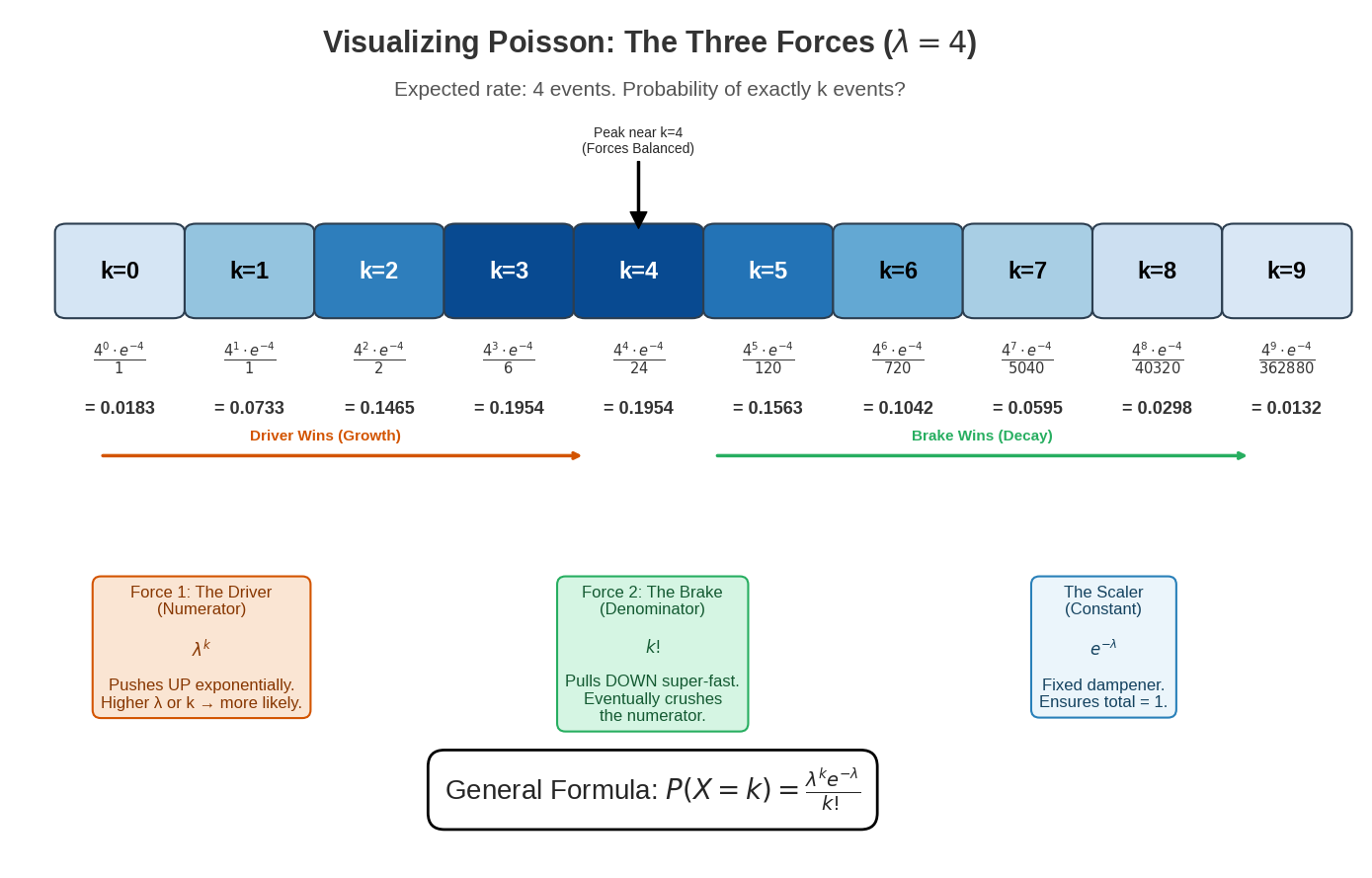
The diagram above visualizes the Poisson distribution (λ = 4) using a three forces metaphor that explains how each component of the formula $P(X=k) = \frac{\lambda^k e^{-\lambda}}{k!}$ shapes the probability distribution:

The Three Forces:

The Driver (Numerator: $\lambda^k$ ) — Shown in the orange box, this force pushes probabilities UP exponentially. As k increases, the numerator grows rapidly when λ is large. This represents the “raw likelihood” of k events based on the rate λ.
The Brake (Denominator: $k!$ ) — Shown in the green box, this force pulls probabilities DOWN super-exponentially. Factorial growth eventually crushes the numerator for large k values, causing the rapid decay in the right tail of the distribution.
The Scaler (Constant: $e^{-\lambda}$ ) — Shown in the blue box, this is a fixed dampening factor that normalizes the distribution to ensure all probabilities sum to 1.

Reading the Diagram:

Color-coded boxes (k=0 through k=9): Darker blue indicates higher probability. Each box shows the formula and exact probability for that k value.
Orange arrow (“Driver Wins”): In the left portion (k < λ), the numerator grows faster than the denominator, causing probabilities to increase.
Green arrow (“Brake Wins”): In the right portion (k > λ), the factorial denominator overwhelms the numerator, causing probabilities to decay rapidly.
Peak indicator: Shows where the forces balance at k ≈ λ, marking the mode of the distribution. For λ = 4, the peak occurs at k = 4 with probability ≈ 0.195 (19.5%).

This “tug-of-war” between the driver and brake forces creates the characteristic bell-like shape of the Poisson distribution, with the peak occurring where these forces are balanced.

Key Characteristics

Scenarios: Emails per hour, customer arrivals per day, typos per page, emergency calls per shift, defects per unit area
Parameter: $\lambda$ , average number of events in the interval ( $\lambda > 0$ )
Random Variable: $X \in \{0, 1, 2, ...\}$

Mean: $E[X] = \lambda$

Variance: $Var(X) = \lambda$

Standard Deviation: $SD(X) = \sqrt{\lambda}$

Note: Mean and variance are equal in a Poisson distribution, so the standard deviation is simply the square root of λ.

Relationship to Other Distributions: The Poisson distribution is an approximation to the Binomial distribution when $n$ is large, $p$ is small, and $\lambda = np$ is moderate. Rule of thumb: use Poisson approximation when $n \ge 20$ and $p \le 0.05$ .

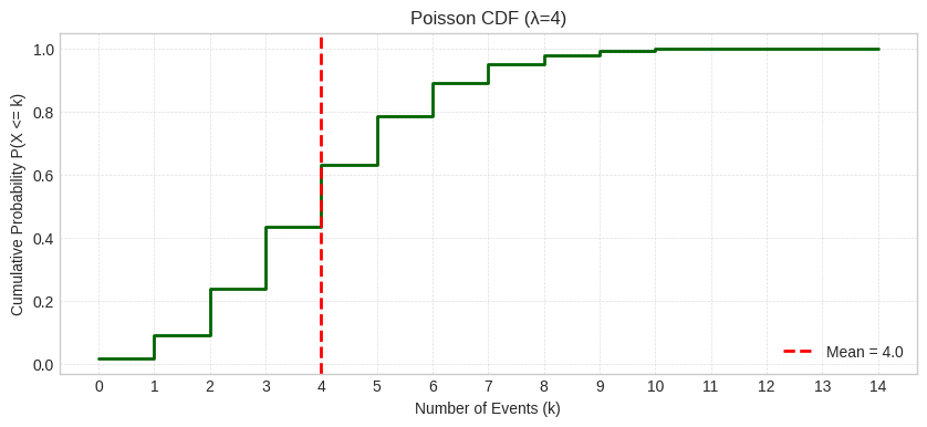
Visualizing the Distribution

Let’s visualize a Poisson distribution with $\lambda = 4$ (our call center example):

# Remove existing SVG if present
if os.path.exists('ch07_poisson_pmf_generic.svg'):
    os.remove('ch07_poisson_pmf_generic.svg')

# Create Poisson distribution for visualization (λ=4)
lambda_viz = 4
poisson_viz = stats.poisson(mu=lambda_viz)

# Calculate mean and std
mean_viz = poisson_viz.mean()
std_viz = poisson_viz.std()

# Plotting the PMF
k_values_viz = np.arange(0, 15)
pmf_values_viz = poisson_viz.pmf(k_values_viz)

plt.figure(figsize=(10, 4))
plt.bar(k_values_viz, pmf_values_viz, color='skyblue', edgecolor='black', alpha=0.7)

# Add mean line
plt.axvline(mean_viz, color='red', linestyle='--', linewidth=2, label=f'Mean = {mean_viz:.1f}')

# Add mean ± 1 std region
plt.axvspan(mean_viz - std_viz, mean_viz + std_viz, alpha=0.2, color='orange',
            label=f'Mean ± 1 SD = [{mean_viz - std_viz:.1f}, {mean_viz + std_viz:.1f}]')

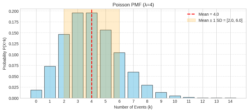
plt.title(f"Poisson PMF (λ={lambda_viz})")
plt.xlabel("Number of Events (k)")
plt.ylabel("Probability P(X=k)")
plt.xticks(k_values_viz)
plt.legend(loc='upper right', fontsize=10)
plt.grid(axis='y', linestyle='--', alpha=0.6)
plt.savefig('ch07_poisson_pmf_generic.svg', format='svg', bbox_inches='tight')
plt.show()

The PMF shows the distribution centered around λ = 4 with reasonable probability for nearby values. The shaded region shows mean ± 1 standard deviation ( $\sqrt{4} = 2$ ).

# Remove existing SVG if present
if os.path.exists('ch07_poisson_cdf_generic.svg'):
    os.remove('ch07_poisson_cdf_generic.svg')

# Plotting the CDF
cdf_values_viz = poisson_viz.cdf(k_values_viz)

plt.figure(figsize=(10, 4))
plt.step(k_values_viz, cdf_values_viz, where='post', color='darkgreen', linewidth=2)

# Add mean line
plt.axvline(mean_viz, color='red', linestyle='--', linewidth=2, label=f'Mean = {mean_viz:.1f}')

plt.title(f"Poisson CDF (λ={lambda_viz})")
plt.xlabel("Number of Events (k)")
plt.ylabel("Cumulative Probability P(X <= k)")
plt.xticks(k_values_viz)
plt.legend(loc='lower right', fontsize=10)
plt.grid(True, which='both', linestyle='--', linewidth=0.5, alpha=0.6)
plt.savefig('ch07_poisson_cdf_generic.svg', format='svg', bbox_inches='tight')
plt.show()

The CDF shows P(X ≤ k), useful for questions like “What’s the probability of 6 or fewer calls?” The red dashed line marks the mean.

Example: Email Arrivals with λ = 5

Modeling the number of emails received per hour with an average rate of λ = 5 emails/hour.

Let’s use scipy.stats.poisson to calculate the probability of observing different numbers of events and verify that the mean equals the variance.

Setting up the distribution:

We create a Poisson distribution with rate parameter λ = 5 (average 5 emails per hour):

import numpy as np
from scipy import stats
import matplotlib.pyplot as plt

# Using scipy.stats.poisson
lambda_rate = 5
poisson_rv = stats.poisson(mu=lambda_rate)

Calculating specific probabilities using the PMF:

What’s the probability of receiving exactly 3 emails in a given hour?

# PMF: Probability of exactly k events
k_events = 3
print(f"P(X={k_events} emails in an hour | lambda={lambda_rate}): {poisson_rv.pmf(k_events):.4f}")

P(X=3 emails in an hour | lambda=5): 0.1404

There’s a 14.04% chance of receiving exactly 3 emails. This is below the mean of 5, so it’s less likely than values closer to 5.

Calculating cumulative probabilities using the CDF:

What’s the probability of receiving 6 or fewer emails in an hour?

# CDF: Probability of k or fewer events
k_or_fewer_events = 6
print(f"P(X <= {k_or_fewer_events} emails in an hour): {poisson_rv.cdf(k_or_fewer_events):.4f}")
print(f"P(X > {k_or_fewer_events} emails in an hour): {1 - poisson_rv.cdf(k_or_fewer_events):.4f}")
print(f"P(X > {k_or_fewer_events} emails in an hour) (using sf): {poisson_rv.sf(k_or_fewer_events):.4f}")

P(X <= 6 emails in an hour): 0.7622
P(X > 6 emails in an hour): 0.2378
P(X > 6 emails in an hour) (using sf): 0.2378

There’s a 76.22% chance of receiving 6 or fewer emails, which means a 23.78% chance of receiving more than 6 emails in an hour.

Verifying the key Poisson property: mean equals variance:

A unique property of the Poisson distribution is that E[X] = Var(X) = λ:

# Mean and Variance
print(f"Mean (Expected number of emails): {poisson_rv.mean():.2f}")
print(f"Variance: {poisson_rv.var():.2f}")

Mean (Expected number of emails): 5.00
Variance: 5.00

As expected, both the mean and variance equal 5.00, confirming the theoretical property of the Poisson distribution.

Generating random samples:

We can simulate many one-hour periods to see the variation in email arrivals:

# Generate random samples
n_simulations = 1000
samples = poisson_rv.rvs(size=n_simulations)
# print(f"\nSimulated number of emails per hour ({n_simulations} simulations): {samples[:20]}...")

These 1000 samples represent different hours, each showing how many emails arrived during that hour.

Visualizing the PMF:

Let’s see the full probability distribution for different email counts:

# Plotting the PMF
k_values = np.arange(0, 16) # Plot for k=0 to 15
pmf_values = poisson_rv.pmf(k_values)

plt.figure(figsize=(8, 3.5))
plt.bar(k_values, pmf_values, color='skyblue', edgecolor='black', alpha=0.7)
plt.title(f"Poisson PMF (λ={lambda_rate})")
plt.xlabel("Number of Events (k)")
plt.ylabel("Probability P(X=k)")
plt.xticks(k_values)
plt.grid(axis='y', linestyle='--', alpha=0.6)
plt.show()

The PMF shows the distribution centered around λ = 5 emails, with highest probabilities at k = 4 and k = 5. The distribution is roughly symmetric for this value of λ. Values far from 5 (like 0-1 or 11+) have very low probabilities. Notice how the probability at k = 3 (which we calculated as 0.1404) appears as a moderate-height bar.

Visualizing the CDF:

The cumulative distribution helps answer questions about ranges of email counts:

# Plotting the CDF
cdf_values = poisson_rv.cdf(k_values)

plt.figure(figsize=(8, 3.5))
plt.step(k_values, cdf_values, where='post', color='darkgreen', linewidth=2)
plt.title(f"Poisson CDF (λ={lambda_rate})")
plt.xlabel("Number of Events (k)")
plt.ylabel("Cumulative Probability P(X <= k)")
plt.xticks(k_values)
plt.grid(True, which='both', linestyle='--', linewidth=0.5, alpha=0.6)
plt.show()

The CDF shows P(X ≤ k), the cumulative probability. We can see that by k = 6, the CDF reaches about 0.76 (matching our earlier calculation of 76.22%), and by k = 10, it’s close to 1.0, meaning it’s very unlikely to receive more than 10 emails in an hour.

Quick Check Questions

A call center receives an average of 12 calls per hour. What distribution models the number of calls in one hour and what is the parameter?

Answer

Poisson distribution with λ = 12 - Events occurring at a constant average rate in a fixed interval.

For a Poisson distribution with λ = 7, what are the mean and variance?

Answer

Mean = 7, Variance = 7 - For Poisson, both equal λ. This is a unique property of the Poisson distribution.

You count the number of typos on a random page of a book. The average is 2 typos per page. Which distribution?

Answer

Poisson with λ = 2 - Counting discrete events (typos) occurring in a fixed space (one page) at a constant average rate.

This fits Poisson’s requirements:

Events happen independently
Constant average rate
Counting occurrences in fixed interval/space

True or False: In a Poisson distribution, the mean can be different from the variance.

Answer

False - A key property of Poisson is that mean = variance = λ.

This property can help you identify when Poisson might not be the best fit. If your data has variance much larger or smaller than the mean, consider other distributions (e.g., Negative Binomial for overdispersion).

When can Poisson approximate Binomial?

Answer

When n is large, p is small, and np is moderate - Specifically:

n ≥ 20 and p ≤ 0.05, or
n ≥ 100 and np ≤ 10

Then Binomial(n, p) ≈ Poisson(λ = np)

Example: Binomial(n=1000, p=0.003) ≈ Poisson(λ=3)

This works because rare events in many trials behave like events occurring at a constant rate.

6. Hypergeometric Distribution¶

The Hypergeometric distribution models the number of successes in a sample drawn without replacement from a finite population. This is different from Binomial, which assumes sampling with replacement (or infinite population).

Concrete Example

You draw 5 cards from a standard deck of 52 cards. How many Aces will you get?

We model this with a random variable $X$ :

$X$ = the number of Aces in the 5-card hand
Population: N = 52 cards total
Successes in population: K = 4 Aces
Sample size: n = 5 cards drawn
$X$ can take values 0, 1, 2, 3, 4 (can’t get more than 4 Aces!)

The Hypergeometric PMF

For sampling without replacement:

P(X=k) = \frac{\binom{K}{k} \binom{N-K}{n-k}}{\binom{N}{n}}

(12)

This is: (ways to choose k successes from K) × (ways to choose n-k failures from N-K) / (total ways to choose n items from N).

Why This Formula Works

The Hypergeometric formula uses counting principles:

$\binom{N}{n}$ (denominator): Total ways to choose $n$ items from $N$ - this is all possible samples
$\binom{K}{k}$ (numerator): Ways to choose $k$ successes from the $K$ successes available
$\binom{N-K}{n-k}$ (numerator): Ways to choose $n-k$ failures from the $N-K$ failures available

Example: Drawing 5 cards hoping for 2 Aces (N=52, K=4, n=5, k=2):

Ways to choose 2 Aces from 4: $\binom{4}{2} = 6$
Ways to choose 3 non-Aces from 48: $\binom{48}{3} = 17,296$
Ways to choose any 5 cards: $\binom{52}{5} = 2,598,960$
Probability: $\frac{6 \times 17,296}{2,598,960} \approx 0.040$

The formula is essentially: (favorable outcomes) / (total possible outcomes) from basic probability, using combinations to count!

Key Characteristics

Scenarios: Cards from a deck, defective items in small batch, tagged fish in sample, jury selection from finite pool
Parameters:
- $N$ : total population size
- $K$ : total number of successes in population
- $n$ : sample size ( $n \le N$ )
Random Variable: $X$ , bounded by $\max(0, n-(N-K)) \le X \le \min(n, K)$

Mean: $E[X] = n \frac{K}{N}$

Variance: $Var(X) = n \frac{K}{N} \left(1 - \frac{K}{N}\right) \left(\frac{N-n}{N-1}\right)$

Standard Deviation: $SD(X) = \sqrt{n \frac{K}{N} \left(1 - \frac{K}{N}\right) \left(\frac{N-n}{N-1}\right)}$

The term $\frac{N-n}{N-1}$ is the finite population correction factor. As $N \to \infty$ , this approaches 1, and Hypergeometric → Binomial with $p = K/N$ .

Visualizing the Distribution

Let’s visualize a Hypergeometric distribution with N=52, K=4, n=5 (our card example):

# Remove existing SVG if present
if os.path.exists('ch07_hypergeometric_pmf_generic.svg'):
    os.remove('ch07_hypergeometric_pmf_generic.svg')

# Create Hypergeometric distribution for visualization (N=52, K=4, n=5)
N_viz = 52
K_viz = 4
n_viz = 5
hypergeom_viz = stats.hypergeom(M=N_viz, n=K_viz, N=n_viz)

# Calculate mean and std
mean_viz = hypergeom_viz.mean()
std_viz = hypergeom_viz.std()

# Plotting the PMF
k_values_viz = np.arange(0, min(n_viz, K_viz) + 1)
pmf_values_viz = hypergeom_viz.pmf(k_values_viz)

plt.figure(figsize=(10, 4))
plt.bar(k_values_viz, pmf_values_viz, color='skyblue', edgecolor='black', alpha=0.7)

# Add mean line
plt.axvline(mean_viz, color='red', linestyle='--', linewidth=2, label=f'Mean = {mean_viz:.2f}')

# Add mean ± 1 std region
plt.axvspan(mean_viz - std_viz, mean_viz + std_viz, alpha=0.2, color='orange',
            label=f'Mean ± 1 SD = [{mean_viz - std_viz:.2f}, {mean_viz + std_viz:.2f}]')

plt.title(f"Hypergeometric PMF (N={N_viz}, K={K_viz}, n={n_viz})")
plt.xlabel("Number of Successes in Sample (k)")
plt.ylabel("Probability P(X=k)")
plt.xticks(k_values_viz)
plt.legend(loc='upper right', fontsize=10)
plt.grid(axis='y', linestyle='--', alpha=0.6)
plt.savefig('ch07_hypergeometric_pmf_generic.svg', format='svg', bbox_inches='tight')

The PMF shows most likely to get 0 Aces (about 0.66 probability), less likely to get 1 or 2. The red dashed line marks the mean, and the orange shaded region shows mean ± 1 standard deviation.

# Remove existing SVG if present
if os.path.exists('ch07_hypergeometric_cdf_generic.svg'):
    os.remove('ch07_hypergeometric_cdf_generic.svg')

# Plotting the CDF
cdf_values_viz = hypergeom_viz.cdf(k_values_viz)

plt.figure(figsize=(10, 4))
plt.step(k_values_viz, cdf_values_viz, where='post', color='darkgreen', linewidth=2)

# Add mean line
plt.axvline(mean_viz, color='red', linestyle='--', linewidth=2, label=f'Mean = {mean_viz:.2f}')

plt.title(f"Hypergeometric CDF (N={N_viz}, K={K_viz}, n={n_viz})")
plt.xlabel("Number of Successes in Sample (k)")
plt.ylabel("Cumulative Probability P(X <= k)")
plt.xticks(k_values_viz)
plt.legend(loc='lower right', fontsize=10)
plt.grid(True, which='both', linestyle='--', linewidth=0.5, alpha=0.6)
plt.savefig('ch07_hypergeometric_cdf_generic.svg', format='svg', bbox_inches='tight')

The CDF shows P(X ≤ k), useful for questions like “What’s the probability of getting at most 1 Ace?” The red dashed line marks the mean.

Example: Lottery Tickets with N=100, K=20, n=10

Modeling the number of winning lottery tickets in a sample of 10 drawn from a box of 100 tickets where 20 are winners.

We’ll use scipy.stats.hypergeom to calculate probabilities for sampling without replacement and see how the mean relates to the population proportion.

Setting up the distribution:

We create a hypergeometric distribution for drawing without replacement:

import numpy as np
from scipy import stats
import matplotlib.pyplot as plt

# Using scipy.stats.hypergeom
N_population = 100
K_successes_pop = 20
n_sample = 10
hypergeom_rv = stats.hypergeom(M=N_population, n=K_successes_pop, N=n_sample)

Calculating specific probabilities using the PMF:

What’s the probability of getting exactly 3 winning tickets when we draw 10?

# PMF: Probability of exactly k successes in the sample
k_successes_sample = 3
print(f"P(X={k_successes_sample} winning tickets in sample of {n_sample}): {hypergeom_rv.pmf(k_successes_sample):.4f}")

P(X=3 winning tickets in sample of 10): 0.2092

There’s a 20.13% chance of getting exactly 3 winners. This is higher than the probability of getting 2 winners because 3 is closer to the expected value (see below).

Calculating cumulative probabilities using the CDF:

What’s the probability of getting 2 or fewer winning tickets?

# CDF: Probability of k or fewer successes in the sample
k_or_fewer_sample = 2
print(f"P(X <= {k_or_fewer_sample} winning tickets in sample): {hypergeom_rv.cdf(k_or_fewer_sample):.4f}")
print(f"P(X > {k_or_fewer_sample} winning tickets in sample): {1 - hypergeom_rv.cdf(k_or_fewer_sample):.4f}")
print(f"P(X > {k_or_fewer_sample} winning tickets in sample) (using sf): {hypergeom_rv.sf(k_or_fewer_sample):.4f}")

P(X <= 2 winning tickets in sample): 0.6812
P(X > 2 winning tickets in sample): 0.3188
P(X > 2 winning tickets in sample) (using sf): 0.3188

There’s a 67.67% chance of getting 2 or fewer winners, which means a 32.33% chance of getting more than 2.

Computing mean and variance:

Let’s verify the mean matches the expected proportion from the population:

# Mean and Variance
print(f"Mean (Expected number of winning tickets in sample): {hypergeom_rv.mean():.2f}")
print(f"Variance: {hypergeom_rv.var():.2f}")
print(f"Standard Deviation: {hypergeom_rv.std():.2f}")
# Theoretical mean: E[X] = n * (K/N) = 10 * (20/100) = 2.0

Mean (Expected number of winning tickets in sample): 2.00
Variance: 1.45
Standard Deviation: 1.21

As expected, the mean is 2.0 winners, which is exactly n × (K/N) = 10 × (20/100) = 10 × 0.2. Since 20% of the population are winners, we expect 20% of our sample to be winners. The finite population correction makes the variance (1.44) smaller than it would be for binomial sampling with replacement.

Generating random samples:

We can simulate many draws of 10 tickets:

# Generate random samples
n_simulations = 1000
samples = hypergeom_rv.rvs(size=n_simulations)
# print(f"\nSimulated number of winning tickets ({n_simulations} simulations): {samples[:20]}...")

These 1000 samples represent different sets of 10 tickets drawn from the box, showing natural variation in outcomes.

Visualizing the PMF:

Let’s see the distribution of possible outcomes when drawing 10 tickets:

# Remove existing SVG if present
if os.path.exists('ch07_hypergeometric_pmf.svg'):
    os.remove('ch07_hypergeometric_pmf.svg')

# Plotting the PMF
# Determine possible k values: max(0, n-(N-K)) <= k <= min(n, K)
min_k = max(0, n_sample - (N_population - K_successes_pop))
max_k = min(n_sample, K_successes_pop)
k_values = np.arange(min_k, max_k + 1)
pmf_values = hypergeom_rv.pmf(k_values)

plt.figure(figsize=(8, 3.5))
plt.bar(k_values, pmf_values, color='skyblue', edgecolor='black', alpha=0.7)
plt.title(f"Hypergeometric PMF (N={N_population}, K={K_successes_pop}, n={n_sample})")
plt.xlabel("Number of Successes in Sample (k)")
plt.ylabel("Probability P(X=k)")
plt.xticks(k_values)
plt.grid(axis='y', linestyle='--', alpha=0.6)
plt.savefig('ch07_hypergeometric_pmf.svg', format='svg', bbox_inches='tight')

The PMF is centered around 2 winners (the expected value), with highest probabilities at 1, 2, and 3 winners. Getting 0 winners or 5+ winners is much less likely. The distribution looks roughly bell-shaped, which is typical for hypergeometric distributions when the sample size is small relative to the population. Notice that k = 3 (which we calculated as 20.13%) appears as one of the tallest bars.

Visualizing the CDF:

The cumulative distribution shows the total probability of getting up to k winners:

# Remove existing SVG if present
if os.path.exists('ch07_hypergeometric_cdf.svg'):
    os.remove('ch07_hypergeometric_cdf.svg')

# Plotting the CDF
cdf_values = hypergeom_rv.cdf(k_values)

plt.figure(figsize=(8, 3.5))
plt.step(k_values, cdf_values, where='post', color='darkgreen', linewidth=2)
plt.title(f"Hypergeometric CDF (N={N_population}, K={K_successes_pop}, n={n_sample})")
plt.xlabel("Number of Successes in Sample (k)")
plt.ylabel("Cumulative Probability P(X <= k)")
plt.xticks(k_values)
plt.grid(True, which='both', linestyle='--', linewidth=0.5, alpha=0.6)
plt.savefig('ch07_hypergeometric_cdf.svg', format='svg', bbox_inches='tight')

The CDF shows the cumulative probability. We can see that P(X ≤ 2) ≈ 0.68 (matching our earlier calculation of 67.67%), and by k = 5, nearly all probability has accumulated (close to 1.0).

Quick Check Questions

You draw 7 cards from a deck of 52. You want to know how many hearts you get. What distribution models this and what are the parameters?

Answer

Hypergeometric with N=52, K=13, n=7 - Sampling without replacement from a finite population (13 hearts in 52 cards).

For a Hypergeometric distribution with N=50, K=10, n=5, what is the expected value (mean)?

Answer

E[X] = n(K/N) = 5 × (10/50) = 1 - Expected number of successes in the sample.

A quality inspector randomly selects 10 products from a batch of 100 (where 15 are defective) without replacement. Which distribution?

Answer

Hypergeometric with N=100, K=15, n=10 - Sampling without replacement from a finite population.

This is NOT Binomial because:

We’re sampling without replacement
The sample size (10) is significant relative to population (100)
Each draw changes the probability for subsequent draws

What’s the key difference between Binomial and Hypergeometric distributions?

Answer

Hypergeometric samples WITHOUT replacement (finite population), while Binomial samples WITH replacement (or assumes infinite population).

Key implications:

Hypergeometric: Trials are NOT independent (each draw affects the next)
Binomial: Trials ARE independent (constant probability p)

Rule of thumb: If N > 20n, Hypergeometric ≈ Binomial because the sample is small relative to the population.

When can Hypergeometric be approximated by Binomial?

Answer

When the population is much larger than the sample - Specifically, when N > 20n.

In this case, Hypergeometric(N, K, n) ≈ Binomial(n, p=K/N)

Example: Drawing 10 cards from a population of 1000 cards. The small sample barely affects the population proportions, so with/without replacement gives nearly identical results.

7. Discrete Uniform Distribution¶

The Discrete Uniform distribution models selecting one outcome from a finite set where all outcomes are equally likely.

Concrete Example

Suppose you roll a fair six-sided die. Each face (1, 2, 3, 4, 5, 6) has an equal probability of appearing.

We model this with a random variable $X$ :

$X$ = the number showing on the die
$X$ can take values 1, 2, 3, 4, 5, 6

The probabilities are:

$P(X = 1) = P(X = 2) = \cdots = P(X = 6) = \frac{1}{6}$

The Discrete Uniform PMF

For a Discrete Uniform distribution on the integers from $a$ to $b$ (inclusive):

P(X=k) = \begin{cases} \frac{1}{b-a+1} & \text{if } k \in \{a, a+1, \ldots, b\} \\ 0 & \text{otherwise} \end{cases}

(13)

For our die example with $a = 1$ and $b = 6$ :

$P(X=k) = \frac{1}{6-1+1} = \frac{1}{6}$ for $k \in \{1, 2, 3, 4, 5, 6\}$

Key Characteristics

Scenarios: Fair die roll, random selection from a list, lottery number selection, random password digit
Parameters:
- $a$ : minimum value (integer)
- $b$ : maximum value (integer, $b \ge a$ )
Random Variable: $X \in \{a, a+1, \ldots, b\}$

Mean: $E[X] = \frac{a+b}{2}$

Variance: $Var(X) = \frac{(b-a+1)^2 - 1}{12}$

Standard Deviation: $SD(X) = \sqrt{\frac{(b-a+1)^2 - 1}{12}}$

Relationship to Other Distributions: The Discrete Uniform distribution is a special case of the Categorical distribution where all $k$ categories have equal probability $p_i = 1/k$ . If outcomes aren’t equally likely, use Categorical instead.

Visualizing the Distribution

Let’s visualize a Discrete Uniform distribution for a fair die ( $a = 1$ , $b = 6$ ):

# Remove existing SVG if present
if os.path.exists('ch07_discrete_uniform_pmf.svg'):
    os.remove('ch07_discrete_uniform_pmf.svg')

# Create Discrete Uniform distribution for visualization (fair die)
a_viz = 1
b_viz = 6
from scipy.stats import randint
# scipy.stats.randint uses [low, high) so we add 1 to b
uniform_viz = randint(low=a_viz, high=b_viz+1)

# Calculate mean and std
mean_viz = uniform_viz.mean()
std_viz = uniform_viz.std()

# Plotting the PMF
k_values_viz = np.arange(a_viz, b_viz+1)
pmf_values_viz = uniform_viz.pmf(k_values_viz)

plt.figure(figsize=(10, 4))
plt.bar(k_values_viz, pmf_values_viz, color='skyblue', edgecolor='black', alpha=0.7)

# Add mean line
plt.axvline(mean_viz, color='red', linestyle='--', linewidth=2, label=f'Mean = {mean_viz:.2f}')

# Add mean ± 1 std region
plt.axvspan(mean_viz - std_viz, mean_viz + std_viz, alpha=0.2, color='orange',
            label=f'Mean ± 1 SD = [{mean_viz - std_viz:.2f}, {mean_viz + std_viz:.2f}]')

plt.title(f"Discrete Uniform PMF (a={a_viz}, b={b_viz})")
plt.xlabel("Outcome")
plt.ylabel("Probability")
plt.ylim(0, 0.25)
plt.xticks(k_values_viz)
plt.legend(loc='upper right', fontsize=10)
plt.grid(axis='y', linestyle='--', alpha=0.6)
plt.savefig('ch07_discrete_uniform_pmf.svg', format='svg', bbox_inches='tight')

The PMF shows six equal bars, each with probability 1/6, representing the fair die. The shaded region shows mean ± 1 standard deviation.

# Remove existing SVG if present
if os.path.exists('ch07_discrete_uniform_cdf.svg'):
    os.remove('ch07_discrete_uniform_cdf.svg')

# Plotting the CDF
cdf_values_viz = uniform_viz.cdf(k_values_viz)

plt.figure(figsize=(10, 4))
plt.step(k_values_viz, cdf_values_viz, where='post', color='darkgreen', linewidth=2)

# Add mean line
plt.axvline(mean_viz, color='red', linestyle='--', linewidth=2, label=f'Mean = {mean_viz:.2f}')

plt.title(f"Discrete Uniform CDF (a={a_viz}, b={b_viz})")
plt.xlabel("Outcome")
plt.ylabel("Cumulative Probability P(X <= k)")
plt.ylim(0, 1.1)
plt.xticks(k_values_viz)
plt.legend(loc='lower right', fontsize=10)
plt.grid(True, which='both', linestyle='--', linewidth=0.5, alpha=0.6)
plt.savefig('ch07_discrete_uniform_cdf.svg', format='svg', bbox_inches='tight')

The CDF increases in equal steps of 1/6 at each value, reaching 1.0 at the maximum value. The red dashed line marks the mean.

Example: Random Selection from 1 to 20

Modeling a random integer selection from 1 to 20, where each number is equally likely to be chosen.

Let’s use scipy.stats.randint to calculate probabilities and generate samples.

Setting up the distribution:

We create a discrete uniform distribution over integers from 1 to 20 (note: scipy.stats.randint uses half-open intervals [low, high)):

import numpy as np
from scipy import stats
import matplotlib.pyplot as plt

# Using scipy.stats.randint (note: uses [low, high) interval)
a_sel = 1
b_sel = 20
uniform_rv = stats.randint(low=a_sel, high=b_sel+1)

Calculating probabilities using the PMF:

Since all values are equally likely, each value has the same probability:

# PMF: Probability of any specific value
k_val = 7
print(f"P(X={k_val}): {uniform_rv.pmf(k_val):.4f}")
print(f"This equals 1/{b_sel-a_sel+1} = {1/(b_sel-a_sel+1):.4f}")

P(X=7): 0.0500
This equals 1/20 = 0.0500

Each of the 20 values has probability 1/20 = 0.05. The value 7 has the same probability as any other value.

Calculating cumulative probabilities using the CDF:

What’s the probability of selecting a number ≤ 10?

# CDF: Probability of k or fewer
k_threshold = 10
print(f"P(X <= {k_threshold}): {uniform_rv.cdf(k_threshold):.4f}")
print(f"P(X > {k_threshold}): {uniform_rv.sf(k_threshold):.4f}")

P(X <= 10): 0.5000
P(X > 10): 0.5000

There’s a 50% chance of selecting 10 or less (values 1-10), and a 50% chance of selecting more than 10 (values 11-20). This makes sense since 10 is the midpoint.

Computing mean and variance:

Let’s verify the mean is at the center of the range:

# Mean and Variance
print(f"Mean (Expected value): {uniform_rv.mean():.2f}")
print(f"Theoretical mean (a+b)/2: {(a_sel+b_sel)/2:.2f}")
print(f"Variance: {uniform_rv.var():.2f}")

Mean (Expected value): 10.50
Theoretical mean (a+b)/2: 10.50
Variance: 33.25

The mean is 10.50, exactly halfway between 1 and 20, as expected from the formula (a+b)/2 = (1+20)/2 = 10.5.

Generating random samples:

Let’s generate 10 random selections:

# Generate random samples
n_samples = 10
samples = uniform_rv.rvs(size=n_samples)
print(f"{n_samples} random selections from 1 to {b_sel}:")
print(samples)

10 random selections from 1 to 20:
[17 13 12 18  1 11 10 10 14 20]

Each sample is an independent random selection, all values equally likely.

Visualizing the PMF:

The PMF visualization shows the defining characteristic of the uniform distribution—perfect equality:

# Remove existing SVG if present
if os.path.exists('ch07_discrete_uniform_pmf_example.svg'):
    os.remove('ch07_discrete_uniform_pmf_example.svg')

# Plotting the PMF
k_values = np.arange(a_sel, b_sel+1)
pmf_values = uniform_rv.pmf(k_values)

plt.figure(figsize=(10, 4))
plt.bar(k_values, pmf_values, color='skyblue', edgecolor='black', alpha=0.7)
plt.title(f"Discrete Uniform PMF (a={a_sel}, b={b_sel})")
plt.xlabel("Value")
plt.ylabel("Probability")
plt.grid(axis='y', linestyle='--', alpha=0.6)
plt.savefig('ch07_discrete_uniform_pmf_example.svg', format='svg', bbox_inches='tight')

All 20 values have equal probability of 0.05 (1/20). This flat distribution is the signature of the discrete uniform—no value is more likely than any other.

Visualizing the CDF:

The CDF shows a perfect linear staircase:

# Remove existing SVG if present
if os.path.exists('ch07_discrete_uniform_cdf_example.svg'):
    os.remove('ch07_discrete_uniform_cdf_example.svg')

# Plotting the CDF
cdf_values = uniform_rv.cdf(k_values)

plt.figure(figsize=(10, 4))
plt.step(k_values, cdf_values, where='post', color='darkgreen', linewidth=2)
plt.title(f"Discrete Uniform CDF (a={a_sel}, b={b_sel})")
plt.xlabel("Value")
plt.ylabel("Cumulative Probability P(X <= k)")
plt.grid(True, which='both', linestyle='--', linewidth=0.5, alpha=0.6)
plt.savefig('ch07_discrete_uniform_cdf_example.svg', format='svg', bbox_inches='tight')

The CDF increases in equal steps of 1/20 = 0.05, perfectly linear. At k=10, the CDF is exactly 0.5 (the median), confirming our earlier calculation.

Quick Check Questions

You randomly select a card from a standard deck (52 cards). If X represents the card number (1-13, where 1=Ace, 11=Jack, 12=Queen, 13=King), what distribution models this and what are the parameters?

Answer

Discrete Uniform distribution with a = 1, b = 13 - Each card number is equally likely (4 of each in the deck).

For a Discrete Uniform distribution with a = 5 and b = 15, what is the probability of getting exactly 10?

Answer

P(X = 10) = 1/(15-5+1) = 1/11 ≈ 0.091 - All values in the range are equally likely.

What is the mean of a Discrete Uniform distribution on the integers from 1 to 100?

Answer

Mean = (1+100)/2 = 50.5 - The mean is the midpoint of the range.

You’re modeling the outcome of rolling a fair six-sided die. Should you use Discrete Uniform or Categorical distribution?

Answer

Discrete Uniform distribution - Since it’s a fair die, all outcomes (1-6) are equally likely with probability 1/6 each.

Use Discrete Uniform(a=1, b=6).

Note: If the die were loaded (unequal probabilities), you’d use the Categorical distribution instead.

For a Discrete Uniform distribution on integers from a to b, why is the variance equal to $\frac{(b-a)(b-a+2)}{12}$ ?

Answer

The variance formula reflects how spread out the values are:

Larger range (b-a): Higher variance - values are more spread out
Formula intuition: The variance grows with the square of the range, similar to continuous uniform distributions

Example:

Discrete Uniform(1, 6): Variance = (6-1)(6-1+2)/12 = 5×7/12 ≈ 2.92
Discrete Uniform(1, 100): Variance = 99×101/12 ≈ 833.25

Much larger range → much larger variance.

8. Categorical Distribution¶

The Categorical distribution models a single trial with multiple possible outcomes (more than 2), where each outcome has its own probability. It’s the generalization of the Bernoulli distribution to more than two categories.

Concrete Example

Suppose you’re rolling a loaded six-sided die where the faces have different probabilities:

Face 1: probability 0.1
Face 2: probability 0.15
Face 3: probability 0.20
Face 4: probability 0.25
Face 5: probability 0.20
Face 6: probability 0.10

We model this with a random variable $X$ :

$X$ = the face that appears
$X$ can take values in $\{1, 2, 3, 4, 5, 6\}$
Each value has its own probability: $P(X=1)=0.1, P(X=2)=0.15,$ etc.

The Categorical PMF

For a Categorical distribution with $k$ possible outcomes and probabilities $p_1, p_2, \ldots, p_k$ where $\sum_{i=1}^k p_i = 1$ :

P(X=i) = p_i \quad \text{for } i = 1, 2, \ldots, k

(14)

For our loaded die example:

$P(X=1) = 0.1,\, P(X=2) = 0.15,\, P(X=3) = 0.20$
$P(X=4) = 0.25,\, P(X=5) = 0.20,\, P(X=6) = 0.10$
Sum: $0.1 + 0.15 + 0.20 + 0.25 + 0.20 + 0.10 = 1.0$ ✓

Key Characteristics

Scenarios: Loaded die, customer choosing from menu categories, survey response (multiple choice), weather outcome (sunny/cloudy/rainy/snowy)
Parameters:
- $k$ : number of categories
- $p_1, p_2, \ldots, p_k$ : probabilities for each category (must sum to 1)
Random Variable: $X \in \{1, 2, \ldots, k\}$

Mean: $E[X] = \sum_{i=1}^k i \cdot p_i$ (weighted average of outcomes)

Variance: $Var(X) = \sum_{i=1}^k i^2 \cdot p_i - \left(\sum_{i=1}^k i \cdot p_i\right)^2$

Relationship to Other Distributions: Categorical generalizes Bernoulli (when $k=2$ ) and is a special case of Discrete Uniform (when all $p_i$ are equal). For multiple trials, use the Multinomial distribution instead.

Visualizing the Distribution

Let’s visualize our loaded die Categorical distribution:

# Remove existing SVG if present
if os.path.exists('ch07_categorical_pmf.svg'):
    os.remove('ch07_categorical_pmf.svg')

# Create Categorical distribution for visualization (loaded die)
probs_viz = np.array([0.1, 0.15, 0.20, 0.25, 0.20, 0.10])
from scipy.stats import rv_discrete
values_viz = np.arange(1, 7)
categorical_viz = rv_discrete(values=(values_viz, probs_viz))

# Plotting the PMF
plt.figure(figsize=(8, 3.5))
plt.bar(values_viz, probs_viz, color='skyblue', edgecolor='black', alpha=0.7)
plt.title("Categorical PMF (Loaded Die)")
plt.xlabel("Outcome")
plt.ylabel("Probability")
plt.ylim(0, 0.3)
plt.xticks(values_viz)
plt.grid(axis='y', linestyle='--', alpha=0.6)
plt.savefig('ch07_categorical_pmf.svg', format='svg', bbox_inches='tight')

The PMF shows the different probabilities for each face of the loaded die.

# Remove existing SVG if present
if os.path.exists('ch07_categorical_cdf.svg'):
    os.remove('ch07_categorical_cdf.svg')

# Plotting the CDF
cdf_values_viz = categorical_viz.cdf(values_viz)

plt.figure(figsize=(8, 3.5))
plt.step(values_viz, cdf_values_viz, where='post', color='darkgreen', linewidth=2)
plt.title("Categorical CDF (Loaded Die)")
plt.xlabel("Outcome")
plt.ylabel("Cumulative Probability P(X <= k)")
plt.ylim(0, 1.1)
plt.xticks(values_viz)
plt.grid(True, which='both', linestyle='--', linewidth=0.5, alpha=0.6)
plt.savefig('ch07_categorical_cdf.svg', format='svg', bbox_inches='tight')

The CDF increases by different amounts at each value, reflecting the varying probabilities.

Example: Customer Product Choice

A coffee shop tracks customer drink preferences: 40% choose coffee, 30% choose tea, 20% choose juice, and 10% choose water.

Let’s model this using a Categorical distribution with scipy.stats.rv_discrete.

Setting up the distribution:

We create a categorical distribution with custom probabilities for each category:

import numpy as np
from scipy import stats
import matplotlib.pyplot as plt

# Define the categorical distribution
choices = np.array([1, 2, 3, 4])  # 1=Coffee, 2=Tea, 3=Juice, 4=Water
probs = np.array([0.40, 0.30, 0.20, 0.10])
categorical_rv = stats.rv_discrete(values=(choices, probs))

Displaying probabilities:

Let’s see the probability of each drink choice:

# PMF: Probability of each choice
labels = ['Coffee', 'Tea', 'Juice', 'Water']
for i, (choice, label) in enumerate(zip(choices, labels)):
    print(f"P(X={choice}) [{label}]: {probs[i]:.2f}")

P(X=1) [Coffee]: 0.40
P(X=2) [Tea]: 0.30
P(X=3) [Juice]: 0.20
P(X=4) [Water]: 0.10

Coffee is the most likely choice (40%), followed by tea (30%), juice (20%), and water (10%). Unlike the uniform distribution, these probabilities differ.

Calculating cumulative probabilities:

What’s the probability a customer chooses coffee or tea (categories 1 or 2)?

# CDF: Probability of choice i or lower
print(f"P(X <= 2) [Coffee or Tea]: {categorical_rv.cdf(2):.2f}")
print(f"P(X > 2) [Juice or Water]: {1 - categorical_rv.cdf(2):.2f}")

P(X <= 2) [Coffee or Tea]: 0.70
P(X > 2) [Juice or Water]: 0.30

There’s a 70% chance the customer chooses coffee or tea, and a 30% chance they choose juice or water.

Computing mean and variance:

While mean and variance are less interpretable for categorical data with arbitrary numbering, scipy can compute them:

# Mean and Variance
print(f"Mean (Expected value): {categorical_rv.mean():.2f}")
print(f"Variance: {categorical_rv.var():.2f}")

Mean (Expected value): 2.00
Variance: 1.00

The mean of 2.00 indicates choices are weighted toward lower category numbers (coffee and tea).

Generating random samples:

Let’s simulate 100 customers and see how many choose each drink:

# Generate random samples
n_customers = 100
samples = categorical_rv.rvs(size=n_customers)
print(f"\nSimulated choices for {n_customers} customers:")
for i, label in enumerate(labels, 1):
    count = np.sum(samples == i)
    print(f"{label}: {count} ({count/n_customers:.1%})")


Simulated choices for 100 customers:
Coffee: 38 (38.0%)
Tea: 35 (35.0%)
Juice: 20 (20.0%)
Water: 7 (7.0%)

The simulated counts should approximate the theoretical probabilities (40%, 30%, 20%, 10%), with some random variation.

Visualizing the PMF:

The bar chart clearly shows the different probabilities for each category:

# Remove existing SVG if present
if os.path.exists('ch07_categorical_pmf_example.svg'):
    os.remove('ch07_categorical_pmf_example.svg')

# Plotting the PMF
plt.figure(figsize=(8, 3.5))
plt.bar(choices, probs, tick_label=labels, color='skyblue', edgecolor='black', alpha=0.7)
plt.title("Categorical PMF (Customer Drink Choice)")
plt.xlabel("Choice")
plt.ylabel("Probability")
plt.ylim(0, 0.5)
plt.grid(axis='y', linestyle='--', alpha=0.6)
plt.savefig('ch07_categorical_pmf_example.svg', format='svg', bbox_inches='tight')

The PMF shows unequal bar heights, distinguishing this from a discrete uniform distribution. Coffee (40%) has the tallest bar, while water (10%) has the shortest, clearly visualizing customer preferences.

# Remove existing SVG if present
if os.path.exists('ch07_categorical_cdf_example.svg'):
    os.remove('ch07_categorical_cdf_example.svg')

# Plotting the CDF
cdf_vals = categorical_rv.cdf(choices)

plt.figure(figsize=(8, 3.5))
plt.step(choices, cdf_vals, where='post', color='darkgreen', linewidth=2)
plt.xticks(choices, labels)
plt.title("Categorical CDF (Customer Drink Choice)")
plt.xlabel("Choice")
plt.ylabel("Cumulative Probability P(X <= k)")
plt.ylim(0, 1.1)
plt.grid(True, which='both', linestyle='--', linewidth=0.5, alpha=0.6)
plt.savefig('ch07_categorical_cdf_example.svg', format='svg', bbox_inches='tight')

The CDF shows cumulative probabilities across the ordered choices.

Quick Check Questions

A traffic light can be red (50%), yellow (10%), or green (40%). What distribution models the color when you arrive at an intersection?

Answer

Categorical distribution with k=3 categories and probabilities p₁=0.5, p₂=0.1, p₃=0.4 - Single trial with three possible outcomes.

For a Categorical distribution with 4 equally likely outcomes, what is P(X = 2)?

Answer

P(X = 2) = 0.25 - For equally likely outcomes, each has probability 1/4.

How is the Categorical distribution related to the Bernoulli distribution?

Answer

Bernoulli is a special case of Categorical with k=2 - When there are only two categories, Categorical reduces to Bernoulli.

Categorical generalizes Bernoulli from 2 outcomes to k outcomes.

You’re observing a single customer’s choice from a menu with 5 items having probabilities [0.3, 0.25, 0.2, 0.15, 0.1]. Should you use Categorical or Multinomial distribution?

Answer

Categorical distribution - You’re observing a single trial (one customer making one choice).

Key distinction:

Categorical: Single trial, multiple outcomes (this scenario)
Multinomial: Multiple trials, counting how many times each outcome occurs

If you observed 100 customers and counted how many chose each item, that would be Multinomial.

When can you model a Categorical distribution as a Discrete Uniform distribution?

Answer

When all k categories have equal probability - If p₁ = p₂ = ... = pₖ = 1/k.

Example:

Rolling a fair die (6 equally likely outcomes): Can use either Categorical(p=[1/6, 1/6, 1/6, 1/6, 1/6, 1/6]) or Discrete Uniform(a=1, b=6)
Rolling a loaded die (unequal probabilities): Must use Categorical

Discrete Uniform is just a special case of Categorical where all probabilities are equal.

9. Multinomial Distribution¶

The Multinomial distribution models performing a fixed number of independent trials where each trial has multiple possible outcomes (more than 2), and we count how many times each outcome occurs. It’s the generalization of the Binomial distribution to more than two categories.

Concrete Example

Suppose you roll a fair six-sided die 20 times. We want to know how many times each face (1, 2, 3, 4, 5, 6) appears.

We model this with a random vector $\mathbf{X} = (X_1, X_2, X_3, X_4, X_5, X_6)$ where:

$X_1$ = number of times face 1 appears
$X_2$ = number of times face 2 appears
... and so on
Constraint: $X_1 + X_2 + X_3 + X_4 + X_5 + X_6 = 20$

The probabilities for a fair die are:

$p_1 = p_2 = p_3 = p_4 = p_5 = p_6 = \frac{1}{6}$

The Multinomial PMF

For $n$ independent trials with $k$ possible outcomes and probabilities $p_1, p_2, \ldots, p_k$ where $\sum_{i=1}^k p_i = 1$ :

P(X_1=x_1, X_2=x_2, \ldots, X_k=x_k) = \frac{n!}{x_1! x_2! \cdots x_k!} \, p_1^{x_1} p_2^{x_2} \cdots p_k^{x_k}

(15)

where $x_1 + x_2 + \cdots + x_k = n$ .

The term $\frac{n!}{x_1! x_2! \cdots x_k!}$ is the multinomial coefficient (see Chapter 3: Permutations of Identical Objects).

For our die example, the probability of getting exactly (3, 4, 2, 5, 4, 2) of each face:

\begin{align} P(X_1=3, X_2=4, X_3=2, X_4=5, X_5=4, X_6=2) &= \frac{20!}{3! \, 4! \, 2! \, 5! \, 4! \, 2!} \left(\frac{1}{6}\right)^{20} \\ &= 1.34 \times 10^{13} \times 3.39 \times 10^{-16} \\ &\approx 0.00454 \end{align}

(16)

Why This Formula Works

The Multinomial formula extends the Binomial idea to multiple categories:

$\frac{n!}{x_1! x_2! \cdots x_k!}$ : The multinomial coefficient counts how many different sequences of $n$ trials produce exactly $x_1$ occurrences of category 1, $x_2$ of category 2, etc.
$p_1^{x_1} p_2^{x_2} \cdots p_k^{x_k}$ : Probability of any specific sequence with those counts

Example: With 3 trials and outcomes (A, A, B):

There are $\frac{3!}{2! \, 1!} = 3$ arrangements: AAB, ABA, BAA
Each has probability $p_A^2 p_B^1$
Combined: $3 \times p_A^2 p_B$

The multinomial coefficient is like the binomial coefficient, but for distributing $n$ items among $k$ categories instead of just 2.

Key Characteristics

Scenarios: Rolling a die n times (counting each face), survey with multiple choice options, customer purchases across product categories, DNA base frequencies in a sequence
Parameters:
- $n$ : number of trials
- $k$ : number of categories
- $p_1, p_2, \ldots, p_k$ : probabilities for each category (must sum to 1)
Random Variables: $X_1, X_2, \ldots, X_k$ where $X_i$ = count for category $i$ , and $\sum_{i=1}^k X_i = n$

Mean for each category: $E[X_i] = n p_i$

Variance for each category: $Var(X_i) = n p_i (1-p_i)$

Relationship to Other Distributions: Multinomial generalizes Binomial (when $k=2$ ) and Categorical (single trial becomes multiple trials). Each individual category count $X_i$ follows a Binomial distribution with parameters $(n, p_i)$ .

Visualizing the Distribution

Multinomial distributions are challenging to visualize since they involve multiple variables. Let’s look at a simple case with $k=3$ categories:

# Remove existing SVG if present
if os.path.exists('ch07_multinomial_marginal.svg'):
    os.remove('ch07_multinomial_marginal.svg')

# Simulate multinomial: rolling a 3-sided die 15 times
n_trials = 15
probs_3 = np.array([1/3, 1/3, 1/3])

# Generate many samples
n_sims = 10000
samples = np.random.multinomial(n_trials, probs_3, size=n_sims)

# Plot distribution of outcomes for Category 1 (marginal distribution)
category_1_counts = samples[:, 0]

plt.figure(figsize=(8, 3.5))
plt.hist(category_1_counts, bins=np.arange(0, n_trials+2)-0.5, density=True,
         color='skyblue', edgecolor='black', alpha=0.7)
plt.title(f"Marginal Distribution of Category 1\n(Multinomial with n={n_trials}, k=3, all p=1/3)")
plt.xlabel("Count for Category 1")
plt.ylabel("Probability")
plt.xticks(range(0, n_trials+1))
plt.grid(axis='y', linestyle='--', alpha=0.6)
plt.savefig('ch07_multinomial_marginal.svg', format='svg', bbox_inches='tight')

The marginal distribution of any single category in a Multinomial distribution is actually a Binomial distribution! Here, Category 1 follows Binomial(n=15, p=1/3).

Connecting to our die example: We simplified to 3 categories for easier visualization, but the same principle applies to our 6-sided die example (n=20 rolls). Each face count would follow Binomial(n=20, p=1/6). The histogram would be similar but centered around 20/6 ≈ 3.33 instead of 15/3 = 5.

Example: Customer Product Purchases

A store tracks purchases across 4 product categories: Electronics (30%), Clothing (25%), Home Goods (25%), Food (20%). We observe 50 customers and count how many purchase from each category.

Let’s use numpy.random.multinomial to work with this distribution.

Setting up parameters and computing expected values:

First, let’s define our multinomial parameters and see what counts we expect:

import numpy as np
from scipy import stats
import matplotlib.pyplot as plt

# Define parameters
n_customers = 50
categories = ['Electronics', 'Clothing', 'Home Goods', 'Food']
probs = np.array([0.30, 0.25, 0.25, 0.20])

# Expected counts
expected_counts = n_customers * probs
print("Expected purchases per category:")
for cat, exp in zip(categories, expected_counts):
    print(f"  {cat}: {exp:.1f}")

Expected purchases per category:
  Electronics: 15.0
  Clothing: 12.5
  Home Goods: 12.5
  Food: 10.0

With 50 customers, we expect 15 to buy Electronics (30%), 12.5 each for Clothing and Home Goods (25%), and 10 for Food (20%).

Generating a single sample:

Let’s simulate one day of 50 customers and see how many purchase from each category:

# Generate one sample (one set of 50 customers)
one_sample = np.random.multinomial(n_customers, probs)
print(f"\nOne simulation of {n_customers} customers:")
for cat, count in zip(categories, one_sample):
    print(f"  {cat}: {count}")
print(f"Total: {np.sum(one_sample)}")


One simulation of 50 customers:
  Electronics: 17
  Clothing: 14
  Home Goods: 10
  Food: 9
Total: 50

Notice that the total is always exactly 50—every customer chooses exactly one category. The individual counts will vary around the expected values due to randomness.

Analyzing the distribution through many simulations:

Let’s simulate many days to understand the variability in each category’s count:

# Generate many samples to see the distribution
n_sims = 10000
samples = np.random.multinomial(n_customers, probs, size=n_sims)

# Compute mean and std for each category
for i, cat in enumerate(categories):
    counts = samples[:, i]
    print(f"{cat}:")
    print(f"  Mean: {np.mean(counts):.2f} (theoretical: {n_customers * probs[i]:.2f})")
    print(f"  Std: {np.std(counts):.2f} (theoretical: {np.sqrt(n_customers * probs[i] * (1-probs[i])):.2f})")

Electronics:
  Mean: 14.94 (theoretical: 15.00)
  Std: 3.23 (theoretical: 3.24)
Clothing:
  Mean: 12.53 (theoretical: 12.50)
  Std: 3.08 (theoretical: 3.06)
Home Goods:
  Mean: 12.51 (theoretical: 12.50)
  Std: 3.11 (theoretical: 3.06)
Food:
  Mean: 10.02 (theoretical: 10.00)
  Std: 2.83 (theoretical: 2.83)

The simulated means should closely match the theoretical values (n × p_i), and the standard deviations follow the binomial formula √(n × p_i × (1-p_i)) since each category’s marginal distribution is binomial.

Visualizing the marginal distributions:

Let’s plot the distribution of counts for each category separately:

# Remove existing SVG if present
if os.path.exists('ch07_multinomial_example.svg'):
    os.remove('ch07_multinomial_example.svg')

# Plot distributions for each category
fig, axes = plt.subplots(2, 2, figsize=(12, 8))
axes = axes.flatten()

for i, (cat, ax) in enumerate(zip(categories, axes)):
    counts = samples[:, i]
    ax.hist(counts, bins=np.arange(0, n_customers+2)-0.5, density=True,
            color='skyblue', edgecolor='black', alpha=0.7)
    ax.axvline(expected_counts[i], color='red', linestyle='--', linewidth=2, label=f'Expected: {expected_counts[i]:.1f}')
    ax.set_title(f"{cat} (p={probs[i]})")
    ax.set_xlabel("Number of Purchases")
    ax.set_ylabel("Probability")
    ax.legend()
    ax.grid(axis='y', linestyle='--', alpha=0.6)

plt.tight_layout()
plt.savefig('ch07_multinomial_example.svg', format='svg', bbox_inches='tight')

Each subplot shows one category’s distribution across 10,000 simulations. The histograms are bell-shaped and centered on the expected values (red dashed lines). Electronics (p=0.30) has the highest expected count (15), while Food (p=0.20) has the lowest (10). Each category’s marginal distribution is binomial with parameters (n=50, p=category probability), but importantly, these counts are NOT independent—they must sum to 50.

Quick Check Questions

You flip a fair coin 30 times and count heads and tails. What distribution models the counts?

Answer

Multinomial distribution with n=30, k=2, and p₁=p₂=0.5 - Or equivalently, Binomial(n=30, p=0.5) for the number of heads, since there are only 2 categories.

When k=2, Multinomial is the same as Binomial.

For a Multinomial distribution with n=100 trials and k=4 equally likely categories, what is the expected count for any one category?

Answer

E[X_i] = n × p_i = 100 × 0.25 = 25 - Each category is expected to appear 25 times.

Since all 4 categories are equally likely, p_i = 1/4 = 0.25 for each.

How is the Multinomial distribution related to the Binomial distribution?

Answer

Binomial is a special case of Multinomial with k=2 - When there are only two categories, Multinomial reduces to Binomial.

Multinomial generalizes Binomial from 2 outcomes to k outcomes across multiple trials.

You roll a die 100 times and count how many times each face (1-6) appears. Should you use Categorical or Multinomial distribution?

Answer

Multinomial distribution - You’re performing multiple trials (100 rolls) and counting how many times each outcome occurs.

Key distinction:

Categorical: Single trial, multiple possible outcomes (one roll)
Multinomial: Multiple trials, counting occurrences of each outcome (100 rolls)

Use Multinomial(n=100, k=6, p=[1/6, 1/6, 1/6, 1/6, 1/6, 1/6]) for a fair die.

In a Multinomial distribution, what is the relationship between the individual category counts X₁, X₂, ..., Xₖ?

Answer

They must sum to n - The constraint is: X₁ + X₂ + ... + Xₖ = n

This is because every trial must result in exactly one category, so the total count across all categories equals the number of trials.

Important implication: The counts are not independent - if you know k-1 of the counts, you can determine the last one.

Example: If n=100 and you know X₁=30, X₂=25, X₃=20 in a k=4 category case, then X₄ must equal 25 (since 30+25+20+25=100).

10. Relationships Between Distributions¶

Understanding the connections between these distributions can deepen insight and provide useful approximations.

Bernoulli as a special case of Binomial: A Binomial distribution with $n=1$ trial ( $Binomial(1, p)$ ) is equivalent to a Bernoulli distribution ( $Bernoulli(p)$ ).
Geometric as a special case of Negative Binomial: A Negative Binomial distribution modeling the number of trials until the first success ( $r=1$ ) ( $NegativeBinomial(1, p)$ ) is equivalent to a Geometric distribution ( $Geometric(p)$ ).
Binomial Approximation to Hypergeometric: If the population size $N$ is much larger than the sample size $n$ (e.g., $N > 20n$ ), then drawing without replacement (Hypergeometric) is very similar to drawing with replacement. In this case, the Hypergeometric( $N, K, n$ ) distribution can be well-approximated by the Binomial( $n, p=K/N$ ) distribution. The finite population correction factor $\frac{N-n}{N-1}$ approaches 1.
Poisson Approximation to Binomial: If the number of trials $n$ in a Binomial distribution is large, and the success probability $p$ is small, such that the mean $\lambda = np$ is moderate, then the Binomial( $n, p$ ) distribution can be well-approximated by the Poisson( $\lambda = np$ ) distribution. This is useful because the Poisson PMF is often easier to compute than the Binomial PMF when $n$ is large. A common rule of thumb is to use this approximation if $n \ge 20$ and $p \le 0.05$ , or $n \ge 100$ and $np \le 10$ .

Example: Poisson approximation to Binomial Consider $Binomial(n=1000, p=0.005)$ . Here $n$ is large, $p$ is small. The mean is $\lambda = np = 1000 \times 0.005 = 5$ . We can approximate this with $Poisson(\lambda=5)$ .

Let’s compare the PMF values of both distributions to see how well the Poisson approximation works in practice.

import numpy as np
from scipy import stats
import matplotlib.pyplot as plt

# Setup distributions
n_binom_approx = 1000
p_binom_approx = 0.005
lambda_approx = n_binom_approx * p_binom_approx

binom_rv_approx = stats.binom(n=n_binom_approx, p=p_binom_approx)
poisson_rv_approx = stats.poisson(mu=lambda_approx)

# Compare PMFs
k_vals_compare = np.arange(0, 15)
binom_pmf = binom_rv_approx.pmf(k_vals_compare)
poisson_pmf = poisson_rv_approx.pmf(k_vals_compare)

print(f"Comparing Binomial(n={n_binom_approx}, p={p_binom_approx}) and Poisson(lambda={lambda_approx:.1f})")
print("k\tBinomial P(X=k)\tPoisson P(X=k)\tDifference")
for k, bp, pp in zip(k_vals_compare, binom_pmf, poisson_pmf):
    print(f"{k}\t{bp:.6f}\t{pp:.6f}\t{abs(bp-pp):.6f}")

Comparing Binomial(n=1000, p=0.005) and Poisson(lambda=5.0)
k	Binomial P(X=k)	Poisson P(X=k)	Difference
0	0.006654	0.006738	0.000084
1	0.033437	0.033690	0.000253
2	0.083929	0.084224	0.000296
3	0.140303	0.140374	0.000071
4	0.175731	0.175467	0.000264
5	0.175908	0.175467	0.000440
6	0.146590	0.146223	0.000367
7	0.104602	0.104445	0.000157
8	0.065245	0.065278	0.000033
9	0.036138	0.036266	0.000128
10	0.017996	0.018133	0.000137
11	0.008139	0.008242	0.000103
12	0.003371	0.003434	0.000063
13	0.001287	0.001321	0.000034
14	0.000456	0.000472	0.000016

# Remove existing SVG if present
if os.path.exists('ch07_poisson_binomial_approximation.svg'):
    os.remove('ch07_poisson_binomial_approximation.svg')

# Plotting the comparison
plt.figure(figsize=(10, 4))
plt.bar(k_vals_compare - 0.2, binom_pmf, width=0.4, label=f'Binomial(n={n_binom_approx}, p={p_binom_approx})', align='center', color='skyblue', edgecolor='black', alpha=0.7)
plt.bar(k_vals_compare + 0.2, poisson_pmf, width=0.4, label=f'Poisson(lambda={lambda_approx:.1f})', align='center', color='lightcoral', edgecolor='black', alpha=0.7)
plt.title("Poisson Approximation to Binomial")
plt.xlabel("Number of Successes (k)")
plt.ylabel("Probability")
plt.xticks(k_vals_compare)
plt.grid(axis='y', linestyle='--', alpha=0.6)
plt.legend()
plt.savefig('ch07_poisson_binomial_approximation.svg', format='svg', bbox_inches='tight')

The chart compares the Binomial(100, 0.03) distribution (blue bars) with the Poisson(3.0) approximation (red bars). The distributions are nearly identical, demonstrating that when n is large and p is small, the Poisson provides an excellent and computationally simpler approximation to the Binomial.

Categorical as generalization of Bernoulli: A Categorical distribution with $k=2$ categories ( $Categorical(p_1, p_2)$ where $p_1 + p_2 = 1$ ) is equivalent to a Bernoulli distribution ( $Bernoulli(p_1)$ ). Categorical extends Bernoulli to handle more than two outcomes in a single trial.
Multinomial as generalization of Binomial: A Multinomial distribution with $k=2$ categories ( $Multinomial(n, p_1, p_2)$ where $p_1 + p_2 = 1$ ) is equivalent to a Binomial distribution ( $Binomial(n, p_1)$ ). Multinomial extends Binomial to count outcomes across more than two categories.
Discrete Uniform as special case of Categorical: A Categorical distribution where all $k$ probabilities are equal ( $p_1 = p_2 = \cdots = p_k = \frac{1}{k}$ ) is a Discrete Uniform distribution on $k$ values. This represents maximum uncertainty about a single trial’s outcome.
Marginal distributions of Multinomial are Binomial: If $(X_1, X_2, \ldots, X_k) \sim Multinomial(n, p_1, p_2, \ldots, p_k)$ , then each individual count $X_i$ follows a Binomial distribution: $X_i \sim Binomial(n, p_i)$ . This makes sense because we’re just counting successes (category $i$ ) vs. failures (all other categories) across $n$ trials.

Summary¶

In this chapter, we explored nine fundamental discrete probability distributions:

Bernoulli: Single trial, two outcomes (Success/Failure).
Binomial: Fixed number of independent trials, counts successes.
Geometric: Number of trials until the first success.
Negative Binomial: Number of trials until a fixed number ( $r$ ) of successes.
Poisson: Number of events in a fixed interval of time/space, given an average rate.
Hypergeometric: Number of successes in a sample drawn without replacement from a finite population.
Discrete Uniform: Single trial where all outcomes are equally likely.
Categorical: Single trial with multiple possible outcomes, each with its own probability.
Multinomial: Fixed number of trials with multiple possible outcomes, counting occurrences of each outcome.

We learned the scenarios each distribution models, their parameters, PMFs, means, and variances. Critically, we saw how to leverage scipy.stats functions (pmf, cdf, rvs, mean, var, std, sf) to perform calculations, generate simulations, and visualize these distributions. We also discussed important relationships, such as:

Bernoulli ↔ Binomial ↔ Categorical ↔ Multinomial (generalizations)
Discrete Uniform as a special case of Categorical
Poisson approximation to Binomial
Binomial approximation to Hypergeometric

Mastering these distributions provides a powerful toolkit for modeling various random phenomena encountered in data analysis, science, engineering, and business. In the next chapters, we will transition to continuous random variables and their corresponding common distributions.

Decision Tree: Choosing the Right Distribution

Use this decision tree to help identify which distribution fits your scenario:

Key Questions to Ask:

How many trials? Single → Bernoulli/Categorical/Discrete Uniform. Fixed number → Binomial/Multinomial/Hypergeometric. Variable → Geometric/Negative Binomial.
How many outcomes per trial? Two → Bernoulli/Binomial/Geometric/Negative Binomial. More than two → Categorical/Multinomial/Discrete Uniform.
With or without replacement? With replacement (or infinite population) → Binomial. Without replacement (finite population) → Hypergeometric.
What are you counting? Successes in fixed trials → Binomial/Multinomial. Trials until success → Geometric/Negative Binomial. Events in interval → Poisson.
Are probabilities equal? Yes → Discrete Uniform. No → Categorical.

Example Applications:

“Flip a coin once” → Bernoulli (single trial, 2 outcomes)
“Flip a coin 10 times, count heads” → Binomial (fixed trials, 2 outcomes, with replacement)
“Roll a die until you get a 6” → Geometric (variable trials, waiting for first success)
“Draw 5 cards from a deck, count hearts” → Hypergeometric (fixed trials, 2 outcomes, without replacement)
“Count customers arriving per hour” → Poisson (events in interval)
“Roll a die once” → Discrete Uniform (single trial, 6 equally likely outcomes)
“Traffic light color when you arrive” → Categorical (single trial, 3 outcomes with different probabilities)
“Roll a die 20 times, count each face” → Multinomial (fixed trials, 6 outcomes)

Exploring Additional Distributions¶

While this chapter covers nine fundamental discrete distributions, many other distributions exist for specialized scenarios. Here’s how to learn about distributions beyond this chapter:

How to Approach Learning a New Distribution:

When you encounter a new distribution, follow these steps:

Understand the Scenario: What real-world process does it model? What makes it different from distributions you already know?
Identify the Parameters: What values define the distribution? (like $n$ and $p$ for Binomial, $\lambda$ for Poisson)
Study the PMF (or PDF for continuous): How are probabilities calculated? What’s the formula?
- PMF = Probability Mass Function (discrete distributions, like those in this chapter)
- PDF = Probability Density Function (continuous distributions, covered in Chapters 8-9)
Learn Key Properties: What are the mean and variance? Are there special characteristics?
Explore Relationships: How does it relate to distributions you already know? Is it a special case or generalization of something familiar?
See Examples: Find concrete examples and visualizations to build intuition.
Practice with Code: Use scipy.stats or similar libraries to work with the distribution hands-on.

Key Resources for Learning About Other Distributions:

Wikipedia - Each distribution has a comprehensive article with a standardized format:
- Definition and scenario
- Parameters and support (possible values)
- PMF formula (discrete) or PDF formula (continuous)
- Mean, variance, and other properties
- Relationships to other distributions
- Examples and applications
- Search for: “[Distribution name] distribution” (e.g., “Beta-Binomial distribution”)
SciPy Documentation - Python’s scipy.stats module includes 100+ distributions:
- Complete reference: https://docs.scipy.org/doc/scipy/reference/stats.html
- Each distribution has: PMF (discrete) or PDF (continuous), CDF, mean, variance, random sampling
- Includes code examples showing how to use each distribution
- Discrete distributions: bernoulli, binom, geom, hypergeom, poisson, nbinom, randint, and many more
Interactive Distribution Explorers:
- Search for “distribution explorer” or “probability distribution visualizer”
- These tools let you adjust parameters and see how distributions change
- Helps build intuition about distribution behavior
Classic Textbooks:
- Introduction to Probability by Bertsekas & Tsitsiklis
- A First Course in Probability by Sheldon Ross
- Probability and Statistics by DeGroot & Schervish
- These provide rigorous treatment with proofs and derivations
Online Resources:
- NIST Engineering Statistics Handbook: Comprehensive reference for common distributions
- Wolfram MathWorld: Mathematical encyclopedia with detailed distribution information
- Stack Exchange (Cross Validated): Q&A site for statistics questions

Examples of Other Discrete Distributions:

Here are some distributions you might encounter that we didn’t cover in detail:

Beta-Binomial: Like Binomial, but the success probability $p$ itself is random (varies from trial to trial)
Logarithmic Distribution: Used in ecology and information theory
Zipf Distribution: Models frequency of words, website visits (follows power law)
Zero-Inflated Poisson: Poisson with extra zeros, common in count data
Conway-Maxwell-Poisson: Generalization of Poisson with extra dispersion parameter
Benford’s Law: Distribution of leading digits in real-world datasets

Finding the Right Distribution:

If you have data or a scenario and need to find which distribution fits:

Identify the process: Single trial? Fixed trials? Waiting time? Events in interval?
Check the support: What values can the random variable take? (e.g., 0/1, non-negative integers, finite range)
Consider the parameters: What aspects of the process can vary? (success probability, rate, sample size, etc.)
Use the decision tree (see below) to narrow down candidates
Test candidate distributions using visualizations and goodness-of-fit tests
Consult domain literature: See what distributions are commonly used in your field

Exercises¶

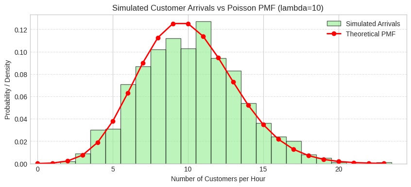
Customer Arrivals: The average number of customers arriving at a small cafe is 10 per hour. Assume arrivals follow a Poisson distribution. a. What is the probability that exactly 8 customers arrive in a given hour? b. What is the probability that 12 or fewer customers arrive in a given hour? c. What is the probability that more than 15 customers arrive in a given hour? d. Simulate 1000 hours of customer arrivals and plot a histogram of the results. Compare it to the theoretical PMF.

Answer

a) Using the Poisson distribution with $\lambda = 10$ :

import numpy as np
from scipy import stats
import matplotlib.pyplot as plt

lambda_cafe = 10
cafe_rv = stats.poisson(mu=lambda_cafe)
prob_8 = cafe_rv.pmf(8)
print(f"P(Exactly 8 customers) = {prob_8:.4f}")

P(Exactly 8 customers) = 0.1126

b) The probability of 12 or fewer customers:

prob_12_or_fewer = cafe_rv.cdf(12)
print(f"P(12 or fewer customers) = {prob_12_or_fewer:.4f}")

P(12 or fewer customers) = 0.7916

c) The probability of more than 15 customers:

prob_over_15 = cafe_rv.sf(15)
print(f"P(More than 15 customers) = {prob_over_15:.4f}")

P(More than 15 customers) = 0.0487

d) Simulation and visualization:

n_sim_hours = 1000
sim_arrivals = cafe_rv.rvs(size=n_sim_hours)

plt.figure(figsize=(10, 4))
max_observed = np.max(sim_arrivals)
bins = np.arange(0, max_observed + 2) - 0.5
plt.hist(sim_arrivals, bins=bins, density=True, alpha=0.6, color='lightgreen', edgecolor='black', label='Simulated Arrivals')

# Overlay theoretical PMF
k_vals_cafe = np.arange(0, max_observed + 1)
pmf_cafe = cafe_rv.pmf(k_vals_cafe)
plt.plot(k_vals_cafe, pmf_cafe, 'ro-', linewidth=2, markersize=6, label='Theoretical PMF')

plt.title(f'Simulated Customer Arrivals vs Poisson PMF (lambda={lambda_cafe})')
plt.xlabel('Number of Customers per Hour')
plt.ylabel('Probability / Density')
plt.legend()
plt.grid(axis='y', linestyle='--', alpha=0.6)
plt.xlim(-0.5, max_observed + 1.5)
plt.show()

The histogram closely matches the theoretical PMF, confirming the Poisson model.

Quality Control: A batch contains 50 items, of which 5 are defective. You randomly sample 8 items without replacement. a. What distribution models the number of defective items in your sample? State the parameters. b. What is the probability that exactly 1 item in your sample is defective? c. What is the probability that at most 2 items in your sample are defective? d. What is the expected number of defective items in your sample?
Answer
a) This follows a Hypergeometric distribution since we’re sampling without replacement from a finite population. The parameters are: $N=50$ (population size), $K=5$ (defective items in population), $n=8$ (sample size).
import numpy as np from scipy import stats import matplotlib.pyplot as plt N_qc = 50 K_qc = 5 n_qc = 8 qc_rv = stats.hypergeom(M=N_qc, n=K_qc, N=n_qc) print(f"Distribution: Hypergeometric(N={N_qc}, K={K_qc}, n={n_qc})")
Distribution: Hypergeometric(N=50, K=5, n=8)
b) Probability of exactly 1 defective item:
```
prob_1_defective = qc_rv.pmf(1)
print(f"P(Exactly 1 defective in sample) = {prob_1_defective:.4f}")
```
P(Exactly 1 defective in sample) = 0.4226
c) Probability of at most 2 defective items:
```
prob_at_most_2 = qc_rv.cdf(2)
print(f"P(At most 2 defectives in sample) = {prob_at_most_2:.4f}")
```
P(At most 2 defectives in sample) = 0.9758
d) Expected number of defective items:
```
expected_defective = qc_rv.mean()
print(f"Expected number of defectives in sample = {expected_defective:.4f}")
# Theoretical: E[X] = n * (K/N) = 8 * (5/50) = 0.8
```
Expected number of defectives in sample = 0.8000

Website Success: A new website feature has a 3% chance of being used by a visitor ( $p=0.03$ ). Assume visitors are independent. a. If 100 visitors come to the site, what is the probability that exactly 3 visitors use the feature? What distribution applies? b. What is the probability that 5 or fewer visitors use the feature out of 100? c. What is the expected number of users out of 100 visitors? d. A developer tests the feature repeatedly until the first user successfully uses it. What is the probability that the first success occurs on the 20th visitor? What distribution applies? e. What is the expected number of visitors needed to see the first success? f. How many visitors are expected until the 5th user is observed? What distribution applies?

Answer

a) This follows a Binomial distribution with $n=100$ trials and $p=0.03$ :

import numpy as np
from scipy import stats
import matplotlib.pyplot as plt

p_ws = 0.03
n_ws = 100
ws_binom_rv = stats.binom(n=n_ws, p=p_ws)
prob_3_users = ws_binom_rv.pmf(3)
print(f"Distribution: Binomial(n={n_ws}, p={p_ws})")
print(f"P(Exactly 3 users) = {prob_3_users:.4f}")

Distribution: Binomial(n=100, p=0.03)
P(Exactly 3 users) = 0.2275

b) Probability of 5 or fewer users:

prob_5_or_fewer = ws_binom_rv.cdf(5)
print(f"P(5 or fewer users) = {prob_5_or_fewer:.4f}")

P(5 or fewer users) = 0.9192

c) Expected number of users:

expected_users = ws_binom_rv.mean()
print(f"Expected number of users = {expected_users:.2f}")
# Theoretical: E[X] = n*p = 100 * 0.03 = 3

Expected number of users = 3.00

d) This follows a Geometric distribution. The probability that the first success occurs on trial 20:

ws_geom_rv = stats.geom(p=p_ws)
prob_first_on_20 = ws_geom_rv.pmf(19)  # scipy counts 19 failures before success
print(f"Distribution: Geometric(p={p_ws})")
print(f"P(First success on trial 20) = {prob_first_on_20:.4f}")

Distribution: Geometric(p=0.03)
P(First success on trial 20) = 0.0173

e) Expected number of visitors until first success:

expected_trials_geom = 1 / p_ws
print(f"Expected visitors until first success = {expected_trials_geom:.2f}")
# Theoretical: E[X] = 1/p = 1/0.03 ≈ 33.33

Expected visitors until first success = 33.33

f) This follows a Negative Binomial distribution with $r=5$ successes:

r_ws = 5
expected_trials_nbinom = r_ws / p_ws
print(f"Distribution: Negative Binomial(r={r_ws}, p={p_ws})")
print(f"Expected visitors until 5th success = {expected_trials_nbinom:.2f}")
# Theoretical: E[X] = r/p = 5/0.03 ≈ 166.67

Distribution: Negative Binomial(r=5, p=0.03)
Expected visitors until 5th success = 166.67