NN02 - Training an Edge-Detection Neural Network from Scratch
A visual guide to how neural networks learn, using edge detection as our example
Neural networks can seem intimidating. Terms like “cross-entropy loss,” “softmax,” and “backpropagation” sound complex. But at their core, these are just clever combinations of simple operations.
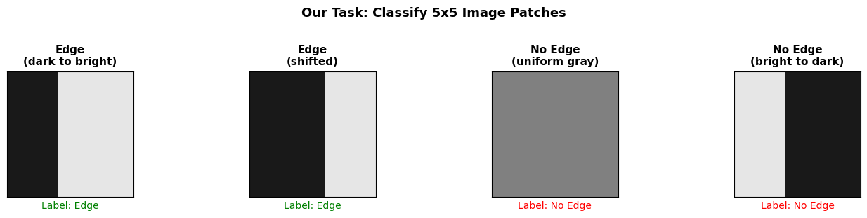
This tutorial explains how neural networks learn — specifically, how they automatically discover the right weights through training. We’ll use edge detection as our running example: training a network to look at a small image patch and answer “Is there a vertical edge here?”
By the end, you’ll understand:
How a neuron detects patterns (like edges)
How we measure “wrongness” with the loss function
How backpropagation computes gradients
How gradient descent learns the right weights
Companion post: For a deeper dive into how a single neuron works as a pattern detector (weights, ReLU, bias), see NN01 - Edge Detection Intuition: A Single Neuron as Pattern Matching. This tutorial focuses on the training process — how the network discovers those weights automatically.
# Setup
import logging
import numpy as np
import warnings

logging.getLogger("matplotlib.font_manager").setLevel(logging.ERROR)

import matplotlib.pyplot as plt
import matplotlib.patches as mpatches

plt.rcParams['figure.facecolor'] = 'white'
plt.rcParams['axes.facecolor'] = 'white'
plt.rcParams['axes.grid'] = False
Let’s trace real numbers through the network to see the big picture. Don’t worry about understanding every detail yet — we’ll explain each concept in the sections that follow:
Part 2: How neurons compute weighted sums and apply ReLU
Part 3: How softmax converts scores to probabilities
Part 4: How the loss function measures “wrongness” — Cross-Entropy
For now, just watch the shapes and values flow through:
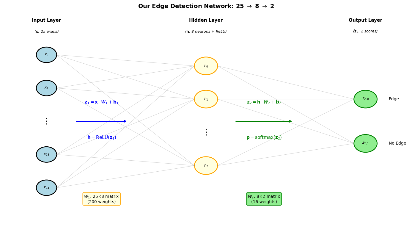
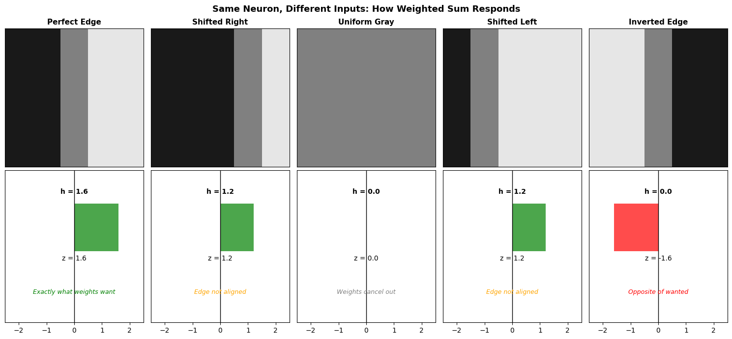
Each input xi (a scalar — one pixel value) is multiplied by its weight wi (also a scalar), all products are summed, and a bias b (scalar) is added. The result z is a single number.
Weights determine how much each input matters
Bias shifts when the neuron “fires”
For one neuron:z=x⋅w+b, where x is the input vector (25 pixels) and w is that neuron’s weight vector (25 weights).
For all neurons at once:z1=x⋅W1+b1, where W1 is a matrix (25×8) — each column is one neuron’s weights. This computes all 8 hidden neurons in one operation!
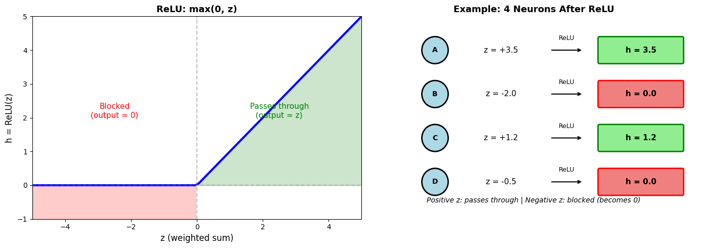
ReLU (Rectified Linear Unit) is the simplest activation:
If z > 0: output z (pass through)
If z ≤ 0: output 0 (block it)
The activation function adds non-linearity. Without it, stacking layers would be pointless — the whole network would just be one big linear equation!
Why non-linearity matters:
The problem with pure linear layers: A linear function always does the same thing to every input: multiply and add. If you chain two linear functions, you still just get multiply and add: z2=(xW1)W2=x(W1W2) — it collapses to a single operation. You can only draw straight lines.
How ReLU fixes this: ReLU makes a decision based on the input:
if z > 0: pass it through
if z ≤ 0: block it (output 0)
This “if/else” behavior is the key! A purely linear function has no “if” — it blindly does the same multiplication regardless of input. ReLU says “it depends on the value.” Different inputs get treated differently.
With many neurons, each making its own if/else decision, the network can carve up the input space into regions, handling each region differently. That’s how it learns complex, non-linear patterns.
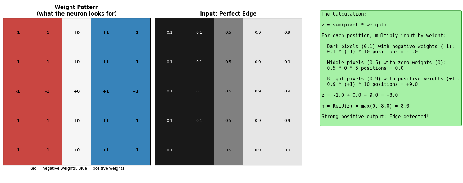
The weights define what pattern the neuron responds to.
The output h is essentially a score for how well the input matches the weight pattern. High score = good match. Zero = no match (or negative match blocked by ReLU).
The chart below shows ReLU in action:
Left: The ReLU function itself — notice how negative values become 0
Right: Four example neurons with different weighted sums (z values). Neurons A and C had positive z, so their outputs pass through. Neurons B and D had negative z, so ReLU blocks them (output = 0).
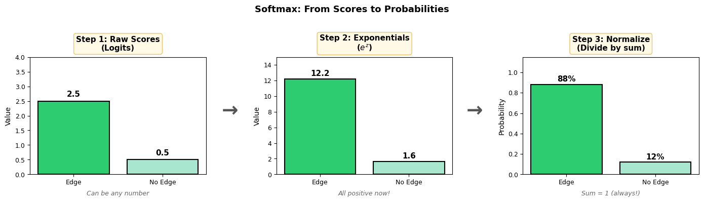
We saw that neurons produce scores — higher means better pattern match. But for classification, we need probabilities: “What’s the chance this is an edge?”
Our network has two output neurons (one for “Edge”, one for “No Edge”), each producing a score. So we have a vector of scoresz=[zedge,zno_edge]. These raw scores can be any number — positive, negative, or zero.
📘 Terminology: Logits
The raw scores before softmax are called logits. You’ll see this term everywhere in machine learning.
Logits can be any real number (−∞ to +∞)
Softmax converts logits → probabilities (0 to 1, summing to 1)
Softmax converts this score vector into a probability vector where:
The exponential also amplifies differences — a score of 5 vs 3 becomes e5 vs e3 (148 vs 20), making the network more confident.
The visualization below shows the 3-step process:
# Show softmax with edge detection example - 3 step process
fig, axes = plt.subplots(1, 3, figsize=(14, 4))

# Example scores for an edge image
scores = np.array([2.5, 0.5])  # [Edge score, No Edge score]
labels = ['Edge', 'No Edge']
colors = ['#2ecc71', '#a8e6cf']  # nicer greens

# Step 1: Raw scores (logits)
ax1 = axes[0]
bars1 = ax1.bar(labels, scores, color=colors, edgecolor='black', linewidth=1.5)
ax1.set_ylabel('Value', fontsize=10)
ax1.set_ylim(0, 4)
for bar, val in zip(bars1, scores):
    ax1.text(bar.get_x() + bar.get_width()/2, val + 0.15, f'{val:.1f}',
             ha='center', fontsize=11, fontweight='bold')
ax1.set_title('Step 1: Raw Scores\n(Logits)', fontsize=11, fontweight='bold',
              bbox=dict(boxstyle='round,pad=0.3', facecolor='#fff9e6', ec='#f0c36d'), y=1.02)
ax1.text(0.5, -0.18, 'Can be any number', ha='center', transform=ax1.transAxes,
         fontsize=9, style='italic', color='#666')
ax1.tick_params(axis='both', labelsize=9)

# Step 2: Exponentials
exp_scores = np.exp(scores)
ax2 = axes[1]
bars2 = ax2.bar(labels, exp_scores, color=colors, edgecolor='black', linewidth=1.5)
ax2.set_ylabel('Value', fontsize=10)
ax2.set_ylim(0, 15)
for bar, val in zip(bars2, exp_scores):
    ax2.text(bar.get_x() + bar.get_width()/2, val + 0.4, f'{val:.1f}',
             ha='center', fontsize=11, fontweight='bold')
ax2.set_title('Step 2: Exponentials\n($e^z$)', fontsize=11, fontweight='bold',
              bbox=dict(boxstyle='round,pad=0.3', facecolor='#fff9e6', ec='#f0c36d'), y=1.02)
ax2.text(0.5, -0.18, 'All positive now!', ha='center', transform=ax2.transAxes,
         fontsize=9, style='italic', color='#666')
ax2.tick_params(axis='both', labelsize=9)

# Step 3: Normalize (the ratio)
probs = exp_scores / np.sum(exp_scores)
ax3 = axes[2]
bars3 = ax3.bar(labels, probs, color=colors, edgecolor='black', linewidth=1.5)
ax3.set_ylabel('Probability', fontsize=10)
ax3.set_ylim(0, 1.15)
for bar, val in zip(bars3, probs):
    ax3.text(bar.get_x() + bar.get_width()/2, val + 0.03, f'{val:.0%}',
             ha='center', fontsize=11, fontweight='bold')
ax3.set_title('Step 3: Normalize\n(Divide by sum)', fontsize=11, fontweight='bold',
              bbox=dict(boxstyle='round,pad=0.3', facecolor='#fff9e6', ec='#f0c36d'), y=1.02)
ax3.text(0.5, -0.18, 'Sum = 1 (always!)', ha='center', transform=ax3.transAxes,
         fontsize=9, style='italic', color='#666')
ax3.tick_params(axis='both', labelsize=9)

plt.suptitle('Softmax: From Scores to Probabilities', fontsize=13, fontweight='bold', y=1.02)
plt.tight_layout()
plt.subplots_adjust(wspace=0.4)

# Add arrows between plots using figure coordinates (after tight_layout)
fig.text(0.328, 0.5, '→', fontsize=28, ha='center', va='center', fontweight='bold', color='#555')
fig.text(0.673, 0.5, '→', fontsize=28, ha='center', va='center', fontweight='bold', color='#555')

plt.show()
Implementation:
# z is a vector of scores (logits) for all classes
z = np.array([2.5, 0.5])            # e.g., [Edge score, No-Edge score]

exp_z = np.exp(z)                   # exponentiate each element
p = exp_z / np.sum(exp_z)           # normalize → probability vector

print(f"Logits z: {z}")             # [2.5, 0.5]
print(f"exp(z):   {exp_z}")         # [12.18, 1.65]
print(f"Probs p:  {p}")             # [0.88, 0.12]
This computes all pj values at once: p[j] = ∑kezkezj
Note: In practice, we subtract the max for numerical stability. This prevents overflow with large scores but gives the same result:
This is called cross-entropy loss. The full formula is L=−∑iyilog(pi).
Think of it as measuring surprise. If you predict 99% chance of rain and it rains, you’re not surprised (low loss). If you predict 1% chance of rain and it rains, you’re very surprised (high loss)! Cross-entropy measures this “surprise” when reality (y) differs from your prediction (p).
Since y is one-hot (all zeros except one 1), the sum simplifies to just −log(pcorrect). We explain this simplification in the Summation Trick callout below.
The zeros kill all terms except the correct class — giving us -\log(p_{correct}).
Implementation:
# p is the probability vector from softmax
# y is the one-hot encoded true label
p = np.array([0.88, 0.12])    # predicted: [P(Edge), P(No Edge)]
y = np.array([1, 0])          # true label: Edge (one-hot)

loss = -np.sum(y * np.log(p)) # cross-entropy

print(f"Predictions p: {p}")           # [0.88, 0.12]
print(f"True label y:  {y}")           # [1, 0]
print(f"Loss:          {loss:.3f}")    # 0.128
The loss is small (0.128) because the network correctly predicted “Edge” with high confidence (88%).
Part 5: Learning - How Do We Find the Right Weights?
So far we’ve assumed the weights are “correct” (negative on left, positive on right). But how does the network learn these weights from scratch?
The answer is gradient descent:
Start with random weights
Measure the loss (how wrong are we?)
Compute the gradient (which direction makes loss smaller?)
Update weights in that direction
Repeat!
We’ve already covered step 2 (the loss function in Part 4). This part explains what gradients are and how we use them (steps 3-4). Part 6 shows how to compute gradients through composed functions (chain rule), and Part 7 puts it all together with backpropagation.
We move opposite to the gradient (downhill), scaled by the learning rate α.
📘 Learning Rate (\alpha)
The learning rate controls how big a step we take with each update:
Too large (\alpha = 1.0): Steps are too big, we overshoot and bounce around, may never converge
Too small (\alpha = 0.0001): Steps are tiny, learning is very slow
Just right: Converges smoothly to a good solution
Think of it like descending a mountain in fog. Large steps might make you miss the valley and end up climbing the other side. Small steps are safe but slow.
Practical advice: Start with \alpha = 0.01 or 0.001 and experiment. If loss explodes or oscillates wildly, reduce it. If loss decreases too slowly, increase it. There’s no universal best value — it depends on your network and data.
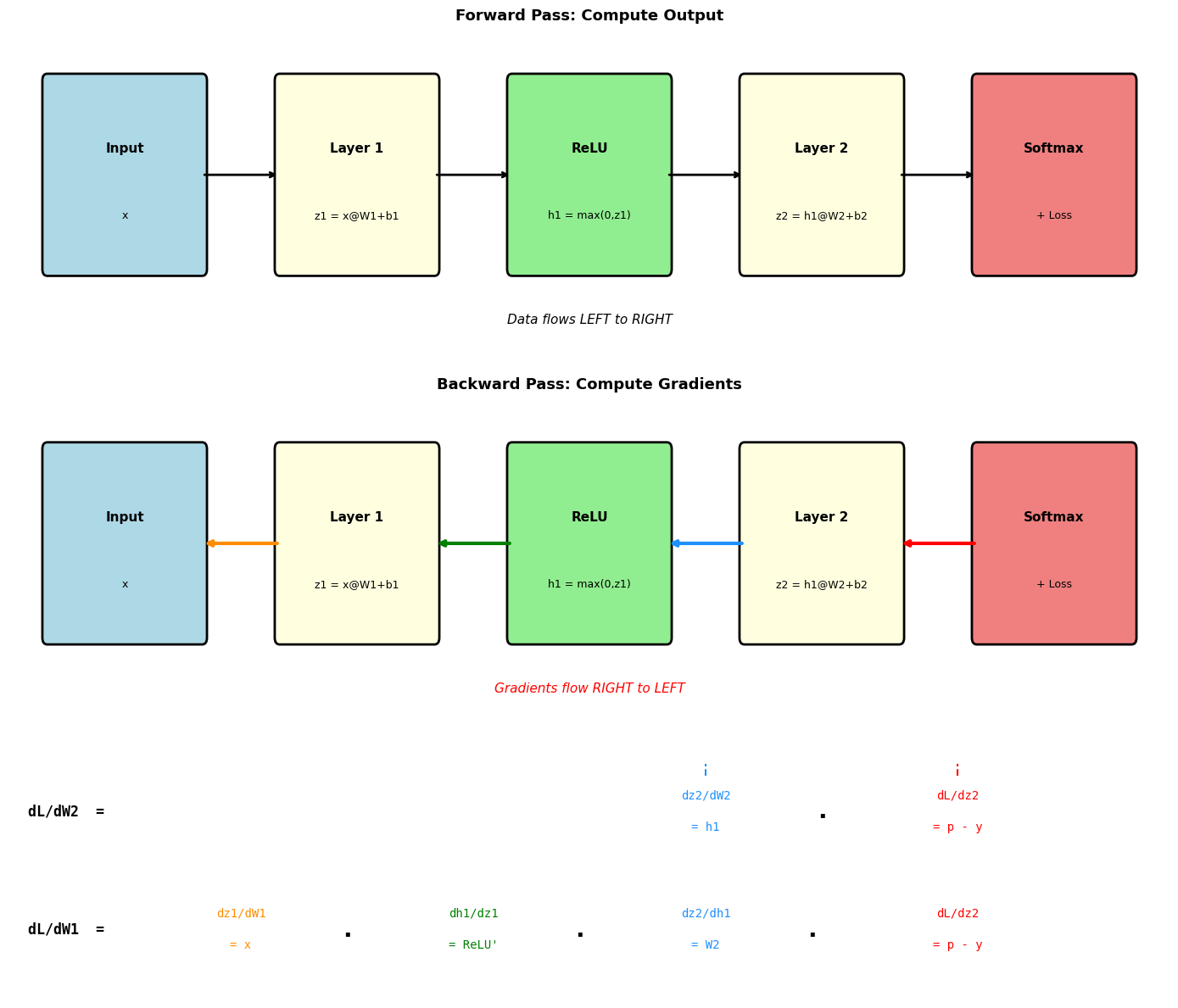
We want to know: how does the loss (a scalar) change when we tweak one weight (also a scalar)? But the weight doesn’t directly affect the loss — it goes through several steps:
This pattern — weight gradient = input × gradient from above — is the core of backpropagation.
Part 7: Backpropagation - Computing Gradients Efficiently
In Part 5, we saw the update rule requires ∂w∂L for each weight. But our network has many weights — how do we compute all these gradients efficiently?
Backpropagation applies the chain rule efficiently using matrix operations. We compute gradients layer by layer, starting from the loss and working backwards.
For a layer with input x (vector), weights W (matrix), and output z (vector):
For our two-layer edge detector (25 → 8 → 2), we compute gradients layer by layer, working backwards from the loss. Each formula below is derived in the Appendix.
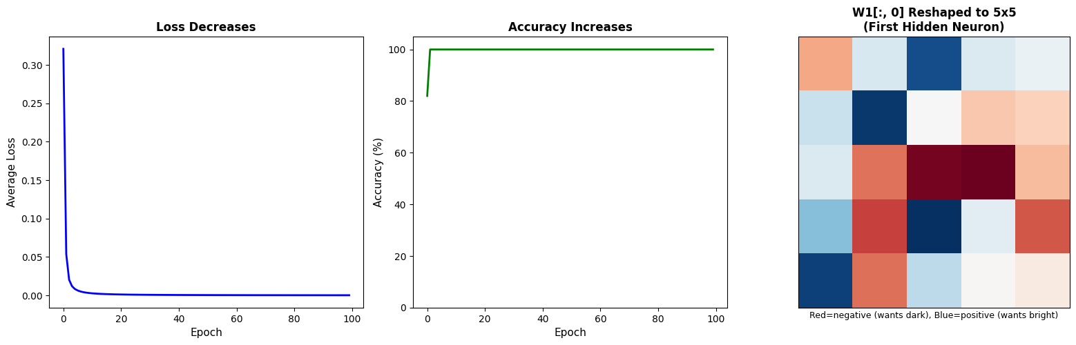
Loss decreased — the network got better at predicting
Accuracy increased — from ~50% (random guessing) to nearly 100%
W1 learned edge patterns — the first hidden neuron’s weights (W1[:, 0] reshaped to 5×5) show the classic edge detector: negative on left, positive on right!
The network discovered the edge detection pattern automatically through gradient descent. We never told it what an edge looks like — it figured it out from examples.
Each of the 8 hidden neurons learns a different pattern. The output layer (W2) then combines these patterns to make the final Edge/No-Edge decision.
Try It Yourself: Complete Edge Detector in ~80 Lines
Here’s a self-contained example with everything we’ve learned: a two-layer network with ReLU activation. It includes data generation, forward pass, backward pass (with backpropagation through both layers), and training.
"""
Complete Neural Network Edge Detector
=====================================
A minimal, self-contained example using only NumPy.
Now with a hidden layer and ReLU!
"""

import numpy as np

# ============================================================
# 1. CREATE TRAINING DATA
# ============================================================
np.random.seed(42)

def make_data(n_samples=100):
    """Generate edge and non-edge image patches."""
    X, y = [], []
    for _ in range(n_samples):
        if np.random.rand() > 0.5:
            # Edge: dark on left, bright on right
            edge_pos = np.random.randint(1, 4)
            patch = np.ones((5, 5)) * 0.1
            patch[:, edge_pos:] = 0.9
            label = [1, 0]  # Edge
        else:
            # No edge: uniform or inverted
            if np.random.rand() > 0.5:
                patch = np.ones((5, 5)) * np.random.uniform(0.3, 0.7)
            else:
                patch = np.ones((5, 5)) * 0.9
                patch[:, 2:] = 0.1  # bright-to-dark (not an edge)
            label = [0, 1]  # No Edge
        X.append(patch.flatten())
        y.append(label)
    return np.array(X), np.array(y)

X_train, y_train = make_data(100)
X_test, y_test = make_data(20)

# ============================================================
# 2. INITIALIZE NETWORK
# ============================================================
# Two-layer network: 25 inputs -> 8 hidden (ReLU) -> 2 outputs
hidden_size = 8

W1 = np.random.randn(25, hidden_size) * 0.3
b1 = np.zeros((1, hidden_size))

W2 = np.random.randn(hidden_size, 2) * 0.3
b2 = np.zeros((1, 2))

learning_rate = 0.1

# ============================================================
# 3. DEFINE FORWARD AND BACKWARD PASS
# ============================================================
def relu(z):
    return np.maximum(0, z)

def relu_derivative(z):
    return (z > 0).astype(float)

def softmax(z):
    exp_z = np.exp(z - np.max(z))
    return exp_z / np.sum(exp_z)

def forward(x):
    """Forward pass through both layers."""
    z1 = x @ W1 + b1           # hidden layer weighted sum
    h1 = relu(z1)              # ReLU activation
    z2 = h1 @ W2 + b2          # output layer weighted sum
    p = softmax(z2)            # softmax probabilities
    return z1, h1, z2, p

def compute_loss(p, y):
    return -np.sum(y * np.log(p + 1e-8))

def backward(x, z1, h1, p, y):
    """Backward pass using the chain rule."""
    # Output layer gradients
    dL_dz2 = p - y                    # softmax + cross-entropy gradient
    dL_dW2 = h1.T @ dL_dz2            # weight gradient = input.T @ gradient
    dL_db2 = dL_dz2

    # Backpropagate through hidden layer
    dL_dh1 = dL_dz2 @ W2.T            # gradient flows back through W2
    dL_dz1 = dL_dh1 * relu_derivative(z1)  # gradient through ReLU
    dL_dW1 = x.T @ dL_dz1             # weight gradient = input.T @ gradient
    dL_db1 = dL_dz1

    return dL_dW1, dL_db1, dL_dW2, dL_db2

# ============================================================
# 4. TRAINING LOOP
# ============================================================
print("Training 2-layer network: 25 -> 8 (ReLU) -> 2")
for epoch in range(100):
    total_loss = 0
    for i in range(len(X_train)):
        x = X_train[i:i+1]
        y = y_train[i:i+1]

        # Forward
        z1, h1, z2, p = forward(x)
        loss = compute_loss(p, y)
        total_loss += loss

        # Backward
        dL_dW1, dL_db1, dL_dW2, dL_db2 = backward(x, z1, h1, p, y)

        # Update all weights
        W1 -= learning_rate * dL_dW1
        b1 -= learning_rate * dL_db1
        W2 -= learning_rate * dL_dW2
        b2 -= learning_rate * dL_db2

    if epoch % 20 == 0:
        print(f"  Epoch {epoch:2d}: Loss = {total_loss/len(X_train):.4f}")

# ============================================================
# 5. EVALUATE ON TEST SET
# ============================================================
correct = 0
for i in range(len(X_test)):
    _, _, _, p = forward(X_test[i:i+1])
    if np.argmax(p) == np.argmax(y_test[i]):
        correct += 1

print(f"\nTest Accuracy: {correct}/{len(X_test)} = {100*correct/len(X_test):.1f}%")

# ============================================================
# 6. EXAMINE WHAT THE NETWORK LEARNED
# ============================================================
print(f"\nHidden layer: {hidden_size} neurons, each looking for a different pattern")
print(f"Output layer: combines hidden features to classify Edge vs No-Edge")
print(f"\nTotal parameters: {25*hidden_size + hidden_size + hidden_size*2 + 2} = {25*hidden_size + hidden_size + hidden_size*2 + 2}")
Training 2-layer network: 25 -> 8 (ReLU) -> 2
  Epoch  0: Loss = 0.1423
Epoch 20: Loss = 0.0005
Epoch 40: Loss = 0.0002
Epoch 60: Loss = 0.0001
Epoch 80: Loss = 0.0001
Test Accuracy: 20/20 = 100.0%

Hidden layer: 8 neurons, each looking for a different pattern
Output layer: combines hidden features to classify Edge vs No-Edge

Total parameters: 226 = 226
Cross-entropy loss measures how wrong we are (Part 4)
The Backward Pass:
4. Gradient descent updates weights opposite to the gradient (Part 5)
5. Chain rule lets us compute derivatives through composed functions (Part 6)
6. Backpropagation efficiently computes all gradients layer by layer (Part 7)
Key Formulas:
Neuron: h=max(0,∑ixiwi+b)
Softmax: pj=∑kezkezj
Cross-entropy: L=−log(pcorrect)
Update: w←w−α∂w∂L
The Magic: By repeating forward-pass, loss, backward-pass, update thousands of times, the network discovers the right weights automatically!
Next Up:Building a Flexible Neural Network — Generalize the code from this tutorial to handle any number of layers, with a clean Layer class abstraction. Same principles, but now you can build networks of any depth!
We need ∂zj∂pi—how changing logit zj affects output pi.
Key insight: Why two indices, i and j?
Unlike simpler functions, softmax couples all outputs—every pi depends on all logits via the denominator ∑kezk. So changing any zj affects every pi, not just pj. We use i and j as two different indices into the same set of classes.
Using the quotient ruledxd[vu]=v2v⋅u′−u⋅v′ with u=ezi and v=∑kezk:
Case 1: When i=j (differentiating pi w.r.t. its own logit zi)