Alternating Least Squares (ALS) for Movie Recommendations

Building a collaborative filtering recommendation system with matrix factorization

Overview¶

This tutorial demonstrates how to build a movie recommendation system using Alternating Least Squares (ALS), a matrix factorization algorithm for collaborative filtering. ALS gained attention during the Netflix Prize era and still provides a clear, interpretable baseline, even though many production systems now favor more sophisticated hybrid or deep-learning approaches.

It is adapted from an older tutorial I wrote around a decade ago on creating a movie recommender with Apache Spark on IBM Bluemix (see movie-recommender-demo), updated here for modern Python workflows and portability.

We’ll explore a MovieLens-style dataset (with some interesting rating biases), visualize the sparsity problem in recommendation systems, and understand how ALS factorizes the user-item rating matrix to make predictions.

import logging
import warnings

logging.getLogger("matplotlib.font_manager").setLevel(logging.ERROR)

import numpy as np
import pandas as pd
import matplotlib.pyplot as plt
import matplotlib.patches as mpatches
from scipy.sparse import csr_matrix
from sklearn.metrics import mean_squared_error

# Configure matplotlib
plt.rcParams['figure.facecolor'] = 'white'
plt.rcParams['axes.facecolor'] = 'white'

Part 1: The Dataset and Sparsity Problem¶

We’ll use the same MovieLens-style ratings dataset from the original Spark tutorial. It includes some interesting biases in how users rate movies, which makes the sparsity patterns more visible.

from pathlib import Path
from urllib.request import urlretrieve

data_url = "https://raw.githubusercontent.com/snowch/movie-recommender-demo/master/web_app/data/ratings.dat"
data_path = Path("data/ratings.dat")
data_path.parent.mkdir(parents=True, exist_ok=True)

if not data_path.exists():
    urlretrieve(data_url, data_path)

ratings = pd.read_csv(
    data_path,
    sep="::",
    engine="python",
    names=["user", "movie", "rating", "timestamp"]
).drop(columns=["timestamp"])

n_users = ratings['user'].max()
n_movies = ratings['movie'].max()
n_ratings = len(ratings)

print(f"Total ratings: {n_ratings}")
print(f"Number of users: {ratings['user'].nunique()}")
print(f"Number of movies: {ratings['movie'].nunique()}")

# Calculate sparsity
total_possible_ratings = n_users * n_movies
sparsity_pct = 100 * (1 - n_ratings / total_possible_ratings)
print(f"\nMatrix sparsity: {sparsity_pct:.2f}%")
print(f"  ({n_ratings:,} ratings out of {total_possible_ratings:,} possible)")

print(f"\nRating distribution:\n{ratings['rating'].value_counts().sort_index()}")

Total ratings: 484560
Number of users: 5384
Number of movies: 2608

Matrix sparsity: 96.90%
  (484,560 ratings out of 15,645,392 possible)

Rating distribution:
rating
1     52817
2     52682
3    126431
4    126127
5    126503
Name: count, dtype: int64

Visualise the ratings matrix using a subset of the data¶

Let’s take a subset of the data.

ratings_subset = ratings.query("user < 20 and movie < 20").copy()
ratings_subset

Separate the x (user) values and also the y (movie) values for matplotlib. Also normalise the rating value so that it is between 0 and 1. This is required for coloring the markers.

user = ratings_subset["user"].astype(int)
movie = ratings_subset["movie"].astype(int)

min_r = ratings_subset["rating"].min()
max_r = ratings_subset["rating"].max()

def normalise(x):
    rating = (x - min_r) / (max_r - min_r)
    return float(rating)

ratingN = ratings_subset["rating"].apply(normalise)

We can now plot the sparse matrix of ratings for this subset of users and movies.

%matplotlib inline
import matplotlib.pyplot as plt
import matplotlib.patches as mpatches
import numpy as np

min_user = ratings_subset["user"].min()
max_user = ratings_subset["user"].max()
min_movie = ratings_subset["movie"].min()
max_movie = ratings_subset["movie"].max()

width = 5
height = 5
plt.figure(figsize=(width, height))
plt.ylim([min_user-1, max_user+1])
plt.xlim([min_movie-1, max_movie+1])
plt.yticks(np.arange(min_user-1, max_user+1, 1))
plt.xticks(np.arange(min_movie-1, max_movie+1, 1))
plt.xlabel('Movie ID')
plt.ylabel('User ID')
plt.title('Movie Ratings')

ax = plt.gca()
ax.patch.set_facecolor('#898787') # dark grey background

colors = plt.cm.YlOrRd(ratingN.to_numpy())

plt.scatter(
    movie.to_numpy(),
    user.to_numpy(),
    s=50,
    marker="s",
    color=colors,
    edgecolor=colors)

plt.legend(
    title='Rating',
    loc="upper left",
    bbox_to_anchor=(1, 1),
    handles=[
        mpatches.Patch(color=plt.cm.YlOrRd(0),    label='1'),
        mpatches.Patch(color=plt.cm.YlOrRd(0.25), label='2'),
        mpatches.Patch(color=plt.cm.YlOrRd(0.5),  label='3'),
        mpatches.Patch(color=plt.cm.YlOrRd(0.75), label='4'),
        mpatches.Patch(color=plt.cm.YlOrRd(0.99), label='5')
    ])

plt.show()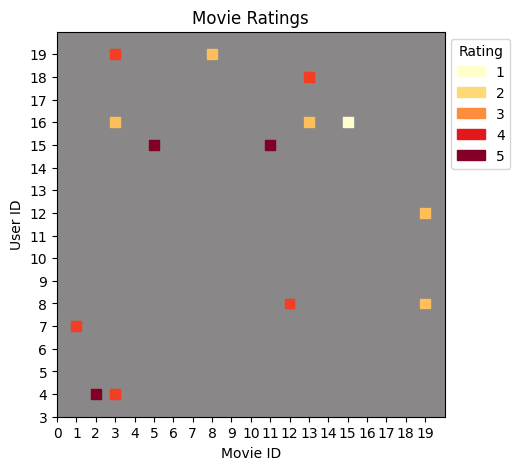

In this plot, you can see how the color coding represents rating values—lighter yellow for low ratings (1-2) and darker red for high ratings (4-5). Each colored square represents a user-movie rating, while the grey background shows positions where no rating exists.

Now that we understand the visualization, let’s apply it to the full dataset.

Visualise the ratings matrix using the full data set¶

This time we don’t need to filter the data.

ratings_full = ratings.copy()

Same functions as before ...

user = ratings_full["user"].astype(int)
movie = ratings_full["movie"].astype(int)

min_r = ratings_full["rating"].min()
max_r = ratings_full["rating"].max()

def normalise(x):
    rating = (x - min_r) / (max_r - min_r)
    return float(rating)

ratingN = ratings_full["rating"].apply(normalise)

Slightly modified chart, for example to print out smaller markers.

%matplotlib inline
import matplotlib.pyplot as plt
import matplotlib.patches as mpatches
import numpy as np

max_user = ratings_full["user"].max()
max_movie = ratings_full["movie"].max()

width = 10
height = 10
plt.figure(figsize=(width, height))
plt.ylim([0, max_user])
plt.xlim([0, max_movie])
plt.ylabel('User ID')
plt.xlabel('Movie ID')
plt.title('Movie Ratings')

ax = plt.gca()
ax.patch.set_facecolor('#898787') # dark grey background

colors = plt.cm.YlOrRd(ratingN.to_numpy())

plt.scatter(
    movie.to_numpy(),
    user.to_numpy(),
    s=1,
    c=colors,
    edgecolors='none',
    alpha=0.6)

plt.legend(
    title='Rating',
    loc="upper left",
    bbox_to_anchor=(1, 1),
    handles=[
        mpatches.Patch(color=plt.cm.YlOrRd(0),    label='1'),
        mpatches.Patch(color=plt.cm.YlOrRd(0.25), label='2'),
        mpatches.Patch(color=plt.cm.YlOrRd(0.5),  label='3'),
        mpatches.Patch(color=plt.cm.YlOrRd(0.75), label='4'),
        mpatches.Patch(color=plt.cm.YlOrRd(0.99), label='5')
    ])

plt.show()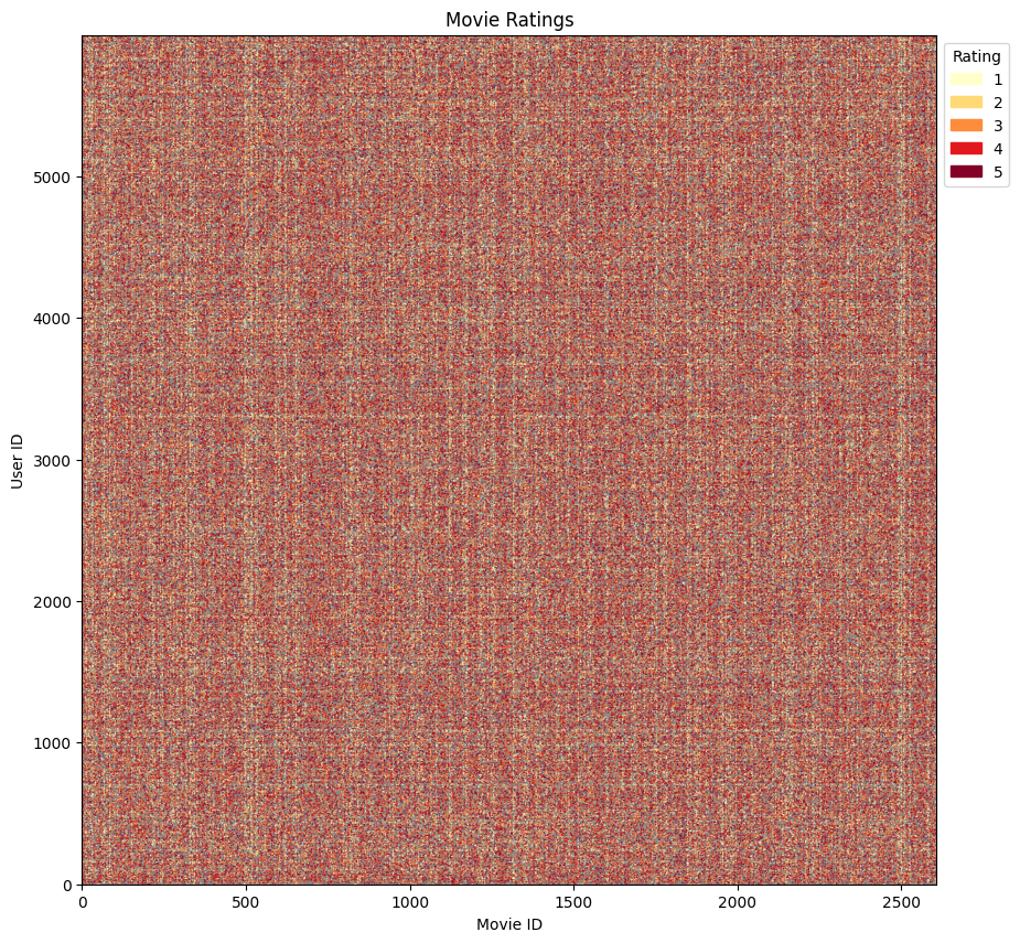

This visualization reveals the fundamental challenge in collaborative filtering: data sparsity. The grey background represents the complete user-item matrix, while colored points show actual ratings. Even though this looks quite dense, the matrix is actually very sparse—most user-movie combinations have no rating.

At this scale with millions of data points compressed into a single visualization, individual patterns are hard to discern. However, there are subtle variations in density that hint at underlying structure:

Some vertical regions have higher density (popular movies rated by many users)
Some horizontal regions show consistent rating patterns (active users)
The transparency reveals areas where ratings are sparser

Key Observation: The matrix is extremely sparse (as calculated above, >95% of potential ratings are missing). The goal of a recommender system is to predict these missing values based on patterns learned from the small fraction of observed ratings.

df = ratings.rename(columns={"user": "user_id", "movie": "movie_id"})

Part 2: The ALS Algorithm¶

The Matrix Factorization Idea¶

ALS solves the recommendation problem by factorizing the user-item rating matrix $R$ (size $m \times n$ ) into two lower-rank matrices:

R \approx U \times M^T

(1)

Where:

$U$ (size $m \times k$ ): User feature matrix—each user represented by $k$ latent factors
$M$ (size $n \times k$ ): Movie feature matrix—each movie represented by $k$ latent factors
$k$ : Number of latent factors (rank), typically $k \ll \min(m, n)$

What Are Latent Factors?¶

Latent factors are hidden features that capture underlying patterns:

For movies: genre preferences, actor preferences, release era, cinematography style
For users: taste in comedy, preference for action, tolerance for violence

Crucially: We don’t specify what these factors mean—the algorithm learns them from data!

Visualizing the Factorization¶

The diagram below illustrates how ALS decomposes the sparse rating matrix into user and product features:

fig = plt.figure(figsize=(16, 7))

# Create main axis for global positioning
ax_main = fig.add_subplot(111)
ax_main.axis('off')

# --- Left: Rating Matrix ---
ax_rating = plt.axes([0.05, 0.25, 0.25, 0.5])

# Create a sample rating matrix (9 users × 8 movies)
n_users_viz, n_movies_viz = 9, 8
rating_matrix_viz = np.full((n_users_viz, n_movies_viz), np.nan)

# Add some sample ratings to highlight
sample_ratings = [
    (0, 1, 5), (1, 1, 5), (4, 4, 2), (5, 1, 4),
    (6, 4, 4), (7, 1, 4), (7, 2, 3), (8, 1, 5)
]

for u, m, r in sample_ratings:
    rating_matrix_viz[u, m] = r

# Plot the rating matrix
im = ax_rating.imshow(np.ones_like(rating_matrix_viz), cmap='Greys', alpha=0.1,
                       aspect='auto', extent=[0.5, n_movies_viz+0.5, n_users_viz+0.5, 0.5])

# Draw grid
for i in range(n_users_viz + 1):
    ax_rating.axhline(i + 0.5, color='gray', linewidth=0.5)
for j in range(n_movies_viz + 1):
    ax_rating.axvline(j + 0.5, color='gray', linewidth=0.5)

# Highlight filled cells with yellow background
for u, m, r in sample_ratings:
    rect = plt.Rectangle((m + 0.5, u + 0.5), 1, 1,
                          facecolor='yellow', edgecolor='orange', linewidth=1.5)
    ax_rating.add_patch(rect)
    ax_rating.text(m + 1, u + 1, str(int(r)), ha='center', va='center',
                   fontsize=11, fontweight='bold', color='blue')

# Add labels
ax_rating.set_xlim(0.5, n_movies_viz + 0.5)
ax_rating.set_ylim(n_users_viz + 0.5, 0.5)
ax_rating.set_xticks(range(1, n_movies_viz + 1))
ax_rating.set_xticklabels(range(1, n_movies_viz + 1))
ax_rating.set_yticks(range(1, n_users_viz + 1))
ax_rating.set_yticklabels(range(1, n_users_viz + 1))
ax_rating.set_xlabel('Item (movie) ID', fontsize=10, fontweight='bold')
ax_rating.set_ylabel('User ID', fontsize=10, fontweight='bold')
ax_rating.set_title('Rating Matrix\n(Sparse)', fontsize=11, fontweight='bold')

# --- Middle: Approximation symbol ---
ax_main.text(0.33, 0.5, '≈', fontsize=50, ha='center', va='center',
             transform=fig.transFigure, fontweight='bold')

# --- Right Top: User Features ---
ax_user = plt.axes([0.40, 0.55, 0.12, 0.2])
n_factors_viz = 5

# Highlight one user (user 1)
user_features_viz = np.full((n_users_viz, n_factors_viz), np.nan)
user_features_viz[0, :] = 1  # User 1 features

im_user = ax_user.imshow(np.ones_like(user_features_viz), cmap='Greys', alpha=0.1,
                          aspect='auto', extent=[0.5, n_factors_viz+0.5, n_users_viz+0.5, 0.5])

# Draw grid
for i in range(n_users_viz + 1):
    ax_user.axhline(i + 0.5, color='gray', linewidth=0.5)
for j in range(n_factors_viz + 1):
    ax_user.axvline(j + 0.5, color='gray', linewidth=0.5)

# Highlight User 1 row
for f in range(n_factors_viz):
    rect = plt.Rectangle((f + 0.5, 0.5), 1, 1,
                          facecolor='lightblue', edgecolor='blue', linewidth=1.5)
    ax_user.add_patch(rect)
    ax_user.text(f + 1, 1, '???', ha='center', va='center',
                 fontsize=9, fontweight='bold', color='blue')

ax_user.set_xlim(0.5, n_factors_viz + 0.5)
ax_user.set_ylim(n_users_viz + 0.5, 0.5)
ax_user.set_xticks(range(1, n_factors_viz + 1))
ax_user.set_xticklabels([f'F{i}' for i in range(1, n_factors_viz + 1)], fontsize=9)
ax_user.set_yticks([1, n_users_viz])
ax_user.set_yticklabels(['1', '...'], fontsize=9)
ax_user.tick_params(left=False, bottom=False)
ax_user.set_title('User Features', fontsize=10, fontweight='bold')

# --- Right Bottom: Product Features ---
ax_product = plt.axes([0.40, 0.25, 0.12, 0.2])

# Highlight one product (product 1)
product_features_viz = np.full((n_factors_viz, n_movies_viz), np.nan)
product_features_viz[:, 0] = 1  # Product 1 features

im_prod = ax_product.imshow(np.ones_like(product_features_viz), cmap='Greys', alpha=0.1,
                             aspect='auto', extent=[0.5, n_movies_viz+0.5, n_factors_viz+0.5, 0.5])

# Draw grid
for i in range(n_factors_viz + 1):
    ax_product.axhline(i + 0.5, color='gray', linewidth=0.5)
for j in range(n_movies_viz + 1):
    ax_product.axvline(j + 0.5, color='gray', linewidth=0.5)

# Highlight Product 1 column
for f in range(n_factors_viz):
    rect = plt.Rectangle((0.5, f + 0.5), 1, 1,
                          facecolor='lightgreen', edgecolor='green', linewidth=1.5)
    ax_product.add_patch(rect)
    ax_product.text(1, f + 1, '???', ha='center', va='center',
                    fontsize=9, fontweight='bold', color='green')

ax_product.set_xlim(0.5, n_movies_viz + 0.5)
ax_product.set_ylim(n_factors_viz + 0.5, 0.5)
ax_product.set_xticks([1, n_movies_viz])
ax_product.set_xticklabels(['1', '...'], fontsize=9)
ax_product.set_yticks(range(1, n_factors_viz + 1))
ax_product.set_yticklabels([f'F{i}' for i in range(1, n_factors_viz + 1)], fontsize=9)
ax_product.tick_params(left=False, bottom=False)
ax_product.set_title('Product Features', fontsize=10, fontweight='bold')

# --- Explanatory Text Box ---
explanation = (
    "This example assumes there are 5 latent\n"
    "factors (F1 to F5) and the job of ALS is to\n"
    "find their values (shown as ???).\n\n"
    "It is our job to experiment to find the\n"
    "optimum number of latent factors."
)

ax_main.text(0.72, 0.5, explanation, fontsize=10, ha='left', va='center',
             transform=fig.transFigure,
             bbox=dict(boxstyle='round,pad=0.8', facecolor='lightyellow',
                      edgecolor='orange', linewidth=2))

plt.show()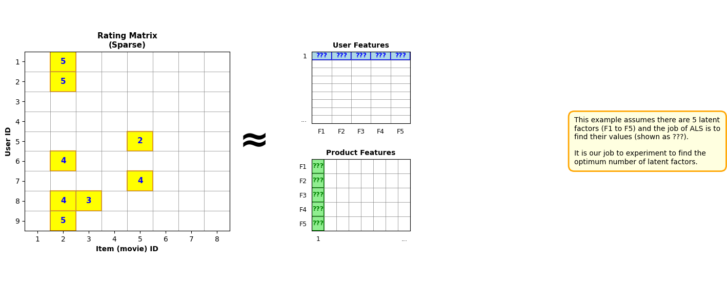

Understanding the Diagram:

The yellow highlighted cells in the Rating Matrix (left) represent observed ratings from users. The grey cells are missing ratings that we want to predict.

ALS decomposes this sparse matrix into:

User Features (top right): Each user is represented by $k$ latent factors (F1-F5 in this example)
Product Features (bottom right): Each movie is represented by the same $k$ latent factors

The “???” symbols indicate that these values are unknown and will be learned by the ALS algorithm.

How ALS Works: The Algorithm¶

ALS alternates between optimizing user factors and movie factors. Here’s how it works:

1. Initialize - Generate small random values for both $U$ (user features) and $M$ (movie features)

2. Fix $M$ , solve for $U$ - Keeping movie features constant, optimize each user’s features using least squares:

U_i = (M^T M + \lambda I)^{-1} M^T R_i

(2)

Where $R_i$ is the vector of ratings from user $i$ (only for movies they rated)

3. Fix $U$ , solve for $M$ - Keeping user features constant, optimize each movie’s features using least squares:

M_j = (U^T U + \lambda I)^{-1} U^T R_j

(3)

Where $R_j$ is the vector of ratings for movie $j$ (only from users who rated it)

4. Repeat - Alternate between steps 2 and 3 for a fixed number of iterations

After each iteration, the reconstruction error (RMSE) decreases as the model learns better representations. The convergence pattern can be visualized in the training curve shown later in this tutorial.

Key Parameters¶

Number of Latent Factors ( $k$ , also called rank):

Determines the dimensionality of the feature space (typically 5-50)
Too few factors: Model may be too simple and underfit the data
Too many factors: Model may overfit and not generalize well
Finding the optimum: Experiment with different values and evaluate on a validation set

It may help intuitively if you think of latent features as representing movie attributes such as genre, actors, or release date—though the algorithm discovers these patterns automatically.

Regularization Parameter ( $\lambda$ ):

Prevents overfitting by adding a penalty term (typically 0.01-0.1)
Why it’s needed: If ALS just solved using pure least squares, the generated User and Product features could be overfitted to the training data
How it works: The $\lambda I$ term in the equations above adds regularization
Finding the optimum: Experiment with different values (try 0.01, 0.05, 0.1, 0.5)

Number of Iterations:

How many times to alternate between solving user and product features (typically 10-20)
More iterations: Generally better fit, but diminishing returns after a certain point
Stopping criteria: Monitor the training error—when it plateaus, additional iterations provide little benefit

Part 3: Implementing ALS from Scratch¶

Let’s implement a simple version of ALS in NumPy:

class SimpleALS:
    """Simplified ALS implementation for collaborative filtering."""

    def __init__(self, n_factors=5, n_iterations=10, lambda_reg=0.1):
        self.n_factors = n_factors
        self.n_iterations = n_iterations
        self.lambda_reg = lambda_reg

    def fit(self, ratings_df):
        """
        Train the ALS model.

        Parameters:
        -----------
        ratings_df : DataFrame with columns [user_id, movie_id, rating]
        """
        # Create user and movie ID mappings
        self.user_ids = ratings_df['user_id'].unique()
        self.movie_ids = ratings_df['movie_id'].unique()
        self.n_users = len(self.user_ids)
        self.n_movies = len(self.movie_ids)

        self.user_id_map = {uid: idx for idx, uid in enumerate(self.user_ids)}
        self.movie_id_map = {mid: idx for idx, mid in enumerate(self.movie_ids)}

        # Create rating matrix (dense for simplicity - production systems use sparse matrices)
        self.R = np.zeros((self.n_users, self.n_movies))
        for _, row in ratings_df.iterrows():
            u_idx = self.user_id_map[row['user_id']]
            m_idx = self.movie_id_map[row['movie_id']]
            self.R[u_idx, m_idx] = row['rating']

        # Initialize user and movie factors
        self.U = np.random.rand(self.n_users, self.n_factors) * 0.01
        self.M = np.random.rand(self.n_movies, self.n_factors) * 0.01

        # Training loop
        self.losses = []
        for iteration in range(self.n_iterations):
            # Fix M, solve for U
            for u in range(self.n_users):
                # Get movies rated by user u
                rated_movies = np.where(self.R[u, :] > 0)[0]
                if len(rated_movies) == 0:
                    continue

                M_u = self.M[rated_movies, :]
                R_u = self.R[u, rated_movies]

                # Solve: U[u] = (M_u^T M_u + λI)^-1 M_u^T R_u
                self.U[u, :] = np.linalg.solve(
                    M_u.T @ M_u + self.lambda_reg * np.eye(self.n_factors),
                    M_u.T @ R_u
                )

            # Fix U, solve for M
            for m in range(self.n_movies):
                # Get users who rated movie m
                rating_users = np.where(self.R[:, m] > 0)[0]
                if len(rating_users) == 0:
                    continue

                U_m = self.U[rating_users, :]
                R_m = self.R[rating_users, m]

                # Solve: M[m] = (U_m^T U_m + λI)^-1 U_m^T R_m
                self.M[m, :] = np.linalg.solve(
                    U_m.T @ U_m + self.lambda_reg * np.eye(self.n_factors),
                    U_m.T @ R_m
                )

            # Calculate loss (RMSE on observed ratings)
            predictions = self.U @ self.M.T
            mask = self.R > 0
            loss = np.sqrt(np.mean((self.R[mask] - predictions[mask]) ** 2))
            self.losses.append(loss)

            if (iteration + 1) % 5 == 0:
                print(f"Iteration {iteration + 1}/{self.n_iterations}, RMSE: {loss:.4f}")

    def predict(self, user_id, movie_id):
        """Predict rating for a user-movie pair."""
        if user_id not in self.user_id_map or movie_id not in self.movie_id_map:
            return np.nan

        u_idx = self.user_id_map[user_id]
        m_idx = self.movie_id_map[movie_id]

        return self.U[u_idx, :] @ self.M[m_idx, :]

    def recommend_top_n(self, user_id, n=5, exclude_rated=True):
        """Get top N movie recommendations for a user."""
        if user_id not in self.user_id_map:
            return []

        u_idx = self.user_id_map[user_id]
        scores = self.U[u_idx, :] @ self.M.T

        if exclude_rated:
            # Exclude movies the user has already rated
            rated_mask = self.R[u_idx, :] > 0
            scores[rated_mask] = -np.inf

        top_indices = np.argsort(scores)[::-1][:n]
        recommendations = [(self.movie_ids[idx], scores[idx]) for idx in top_indices]

        return recommendations

Training the Model¶

First, let’s split the data into training and test sets to properly evaluate the model:

# Split data into train/test (80/20 split)
from sklearn.model_selection import train_test_split

train_df, test_df = train_test_split(df, test_size=0.2, random_state=42)

print(f"Training samples: {len(train_df)}")
print(f"Test samples: {len(test_df)}")

Training samples: 387648
Test samples: 96912

Now train the model on the training set:

# Train the model on training data only
model = SimpleALS(n_factors=10, n_iterations=15, lambda_reg=0.1)
model.fit(train_df)

# Plot training curve
plt.figure(figsize=(10, 6))
plt.plot(range(1, len(model.losses) + 1), model.losses, marker='o', linewidth=2)
plt.xlabel('Iteration', fontsize=12)
plt.ylabel('RMSE', fontsize=12)
plt.title('ALS Training: Loss Over Iterations', fontsize=14, fontweight='bold')
plt.grid(True, alpha=0.3)
plt.tight_layout()
plt.show()

print(f"\nFinal RMSE: {model.losses[-1]:.4f}")

Iteration 5/15, RMSE: 0.6438

Iteration 10/15, RMSE: 0.6278

Iteration 15/15, RMSE: 0.6220


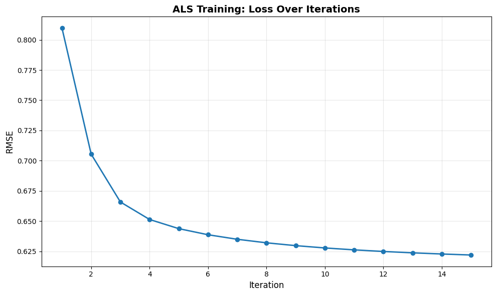
Final RMSE: 0.6220

Part 4: Making Predictions and Recommendations¶

Single Rating Prediction¶

# Example: Predict a specific user-movie rating
user_id = df['user_id'].iloc[0]
movie_id = df['movie_id'].iloc[0]
actual_rating = df[(df['user_id'] == user_id) & (df['movie_id'] == movie_id)]['rating'].values[0]
predicted_rating = model.predict(user_id, movie_id)

print(f"User {user_id}, Movie {movie_id}")
print(f"  Actual rating: {actual_rating}")
print(f"  Predicted rating: {predicted_rating:.2f}")
print(f"  Error: {abs(actual_rating - predicted_rating):.2f}")

User 1, Movie 832
  Actual rating: 2
  Predicted rating: 1.64
  Error: 0.36

Top-N Recommendations¶

# Get top 5 recommendations for a user
user_id = df['user_id'].iloc[0]
recommendations = model.recommend_top_n(user_id, n=5)

print(f"\nTop 5 recommendations for User {user_id}:")
for rank, (movie_id, score) in enumerate(recommendations, 1):
    print(f"  {rank}. Movie {movie_id} (predicted rating: {score:.2f})")


Top 5 recommendations for User 1:
  1. Movie 838 (predicted rating: 2.42)
  2. Movie 1795 (predicted rating: 2.40)
  3. Movie 1039 (predicted rating: 2.34)
  4. Movie 1918 (predicted rating: 2.28)
  5. Movie 353 (predicted rating: 2.27)

Part 5: Understanding the Latent Factors¶

Let’s visualize what the model learned:

fig, (ax1, ax2) = plt.subplots(1, 2, figsize=(14, 5))

# User factors
im1 = ax1.imshow(model.U[:20, :], cmap='coolwarm', aspect='auto')
ax1.set_title('User Latent Factors (First 20 Users)', fontsize=12, fontweight='bold')
ax1.set_xlabel('Latent Factor', fontsize=10)
ax1.set_ylabel('User ID', fontsize=10)
plt.colorbar(im1, ax=ax1, label='Factor Value')

# Movie factors
im2 = ax2.imshow(model.M[:20, :], cmap='coolwarm', aspect='auto')
ax2.set_title('Movie Latent Factors (First 20 Movies)', fontsize=12, fontweight='bold')
ax2.set_xlabel('Latent Factor', fontsize=10)
ax2.set_ylabel('Movie ID', fontsize=10)
plt.colorbar(im2, ax=ax2, label='Factor Value')

plt.tight_layout()
plt.show()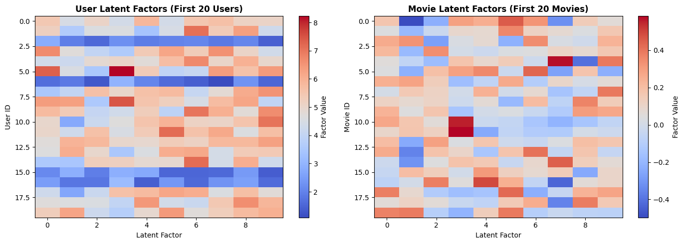

Interpretation:

Positive values (red): User/movie has high affinity for this latent factor
Negative values (blue): User/movie has low affinity for this latent factor
Near zero (white): Neutral

For example, Factor 1 might represent “action movies” while Factor 2 represents “comedy.”

Part 6: Evaluation Metrics¶

Root Mean Squared Error (RMSE)¶

RMSE measures the average prediction error:

\text{RMSE} = \sqrt{\frac{1}{n} \sum_{i=1}^{n} (r_i - \hat{r}_i)^2}

(4)

Where $r_i$ is actual rating and $\hat{r}_i$ is predicted rating.

Interpretation:

RMSE = 0: Perfect predictions
RMSE = 0.5: Predictions off by ~0.5 stars on average
RMSE = 1.0: Predictions off by ~1 star on average

# Evaluate on both training and test sets
def evaluate_model(model, data_df, dataset_name):
    """Calculate RMSE and MAE for a dataset."""
    predictions = []
    actuals = []

    for _, row in data_df.iterrows():
        pred = model.predict(row['user_id'], row['movie_id'])
        if not np.isnan(pred):
            predictions.append(pred)
            actuals.append(row['rating'])

    rmse = np.sqrt(mean_squared_error(actuals, predictions))
    mae = np.mean(np.abs(np.array(actuals) - np.array(predictions)))

    return rmse, mae

# Evaluate on training set
train_rmse, train_mae = evaluate_model(model, train_df, "Training")

# Evaluate on test set (unseen data)
test_rmse, test_mae = evaluate_model(model, test_df, "Test")

print(f"Evaluation Metrics:")
print(f"\nTraining Set:")
print(f"  RMSE: {train_rmse:.4f}")
print(f"  MAE:  {train_mae:.4f}")
print(f"\nTest Set (unseen data):")
print(f"  RMSE: {test_rmse:.4f}")
print(f"  MAE:  {test_mae:.4f}")
print(f"\nInterpretation: On unseen data, predictions are off by ~{test_rmse:.2f} stars on average")
print(f"Overfitting check: {'Minimal overfitting' if (test_rmse - train_rmse) < 0.1 else 'Some overfitting detected'}")

Evaluation Metrics:

Training Set:
  RMSE: 0.6259
  MAE:  0.5207

Test Set (unseen data):
  RMSE: 0.9243
  MAE:  0.7614

Interpretation: On unseen data, predictions are off by ~0.92 stars on average
Overfitting check: Some overfitting detected

Part 7: Key Takeaways¶

Advantages of ALS¶

✅ Scalable: Can handle millions of users and items ✅ Parallelizable: User and movie updates are independent ✅ Interpretable: Latent factors have semantic meaning ✅ Effective: Works well with sparse data

Limitations¶

❌ Cold start problem: Can’t recommend for new users/movies with no ratings ❌ Implicit feedback: Designed for explicit ratings (1-5 stars), not clicks/views ❌ Context-agnostic: Doesn’t consider time, location, or other context

When to Use ALS¶

E-commerce: Product recommendations based on purchase history
Media platforms: Movie/music recommendations (Netflix, Spotify)
Content sites: Article recommendations based on reading patterns
Social networks: Friend or content suggestions

Extensions and Alternatives¶

Implicit ALS: For binary data (clicks, purchases)
Deep Learning: Neural collaborative filtering (NCF)
Hybrid methods: Combine with content-based features
Context-aware: Incorporate temporal or contextual information

Summary¶

We’ve covered:

The Problem: Predicting missing ratings in sparse user-item matrices
The Solution: Matrix factorization using Alternating Least Squares
The Algorithm: Alternating between optimizing user and item factors
Implementation: Building ALS from scratch in NumPy
Evaluation: Using RMSE to measure prediction accuracy
Interpretation: Understanding learned latent factors

Next Steps:

Try on real MovieLens dataset: grouplens.org/datasets/movielens
Experiment with hyperparameters ( $k$ , $\lambda$ , iterations)
Implement implicit feedback version for binary data
Compare with deep learning approaches

References¶

Original Paper: Netflix Prize (2006-2009)
Spark MLlib ALS: Apache Spark Documentation
MovieLens Dataset: GroupLens Research
Source Code: Movie Recommender Demo

This tutorial demonstrates collaborative filtering concepts. For production systems with millions of users, consider using distributed implementations like Spark MLlib, TensorFlow Recommenders, or PyTorch.