Learn how to use Random Forest and XGBoost to identify the most important features in your dataset.
What you’ll learn:
How tree-based models measure feature importance
Using Random Forest and XGBoost for feature selection
Interpreting importance scores
Best practices for feature selection workflows
What is Feature Importance?
The problem: You have a dataset with 100+ features (columns). Which ones actually matter for predicting your target?
Feature importance is a technique to rank features by how much they contribute to a model’s predictions. High-importance features are informative; low-importance features can be dropped to:
Reduce overfitting
Speed up training
Simplify model interpretation
Lower data collection costs
Key insight: Tree-based models (Random Forest, XGBoost) naturally compute feature importance during training as a byproduct of their splitting decisions.
How Tree-Based Models Measure Importance
Decision Tree Basics
A decision tree makes predictions by splitting data at each node:
[Root: All samples]
├─ feature_5 < 0.3?
│  ├─ YES → [Leaf: Class A]
│  └─ NO  → feature_12 < 1.5?
│           ├─ YES → [Leaf: Class B]
│           └─ NO  → [Leaf: Class C]
Key observation: Features used for splits near the root affect more samples and create purer splits. These are the “important” features.
Importance Metrics
1. Gini Importance (Mean Decrease Impurity)
Measures how much each feature reduces impurity (disorder) when used for a split
Higher reduction = more important feature
Default in scikit-learn’s Random Forest
Formula: For each feature, sum the impurity decrease across all trees and all nodes where that feature was used.
2. Permutation Importance
Shuffle a feature’s values and measure how much model accuracy drops
Larger drop = more important feature
More reliable but slower to compute
Using Random Forest for Feature Selection
When to use: You have labeled data and want to quickly identify important features before training a complex model.
import numpy as np
import pandas as pd
from sklearn.ensemble import RandomForestClassifier
from sklearn.datasets import make_classification
import matplotlib.pyplot as plt

# Generate synthetic dataset with 50 features (only 10 informative)
X, y = make_classification(
    n_samples=1000,
    n_features=50,
    n_informative=10,
    n_redundant=5,
    n_clusters_per_class=2,
    random_state=42
)

# Create feature names
feature_names = [f'feature_{i}' for i in range(50)]
df = pd.DataFrame(X, columns=feature_names)
df['target'] = y

print(f"Dataset shape: {df.shape}")
print(f"Features: {len(feature_names)}")
print(f"Truly informative: 10")
Matplotlib is building the font cache; this may take a moment.
Dataset shape: (1000, 51)
Features: 50
Truly informative: 10
Step 1: Train Random Forest
# Train Random Forest
rf = RandomForestClassifier(
    n_estimators=100,  # Number of trees
    max_depth=10,      # Limit depth to prevent overfitting
    random_state=42
)

rf.fit(df[feature_names], df['target'])

# Get feature importances
importances = rf.feature_importances_

# Create DataFrame for easy viewing
importance_df = pd.DataFrame({
    'feature': feature_names,
    'importance': importances
}).sort_values('importance', ascending=False)

print("\nTop 15 most important features:")
print(importance_df.head(15))
Top 15 most important features:
       feature  importance
43  feature_43    0.105803
29  feature_29    0.088805
23  feature_23    0.066776
4    feature_4    0.063832
17  feature_17    0.052174
12  feature_12    0.048990
41  feature_41    0.041088
40  feature_40    0.041085
3    feature_3    0.040936
11  feature_11    0.037626
39  feature_39    0.034435
32  feature_32    0.029210
2    feature_2    0.025263
8    feature_8    0.020942
28  feature_28    0.020856
Step 2: Visualize Importances
# Plot top 20 features
plt.figure(figsize=(10, 6))
top_20 = importance_df.head(20)
plt.barh(range(len(top_20)), top_20['importance'])
plt.yticks(range(len(top_20)), top_20['feature'])
plt.xlabel('Importance Score')
plt.title('Top 20 Feature Importances (Random Forest)')
plt.gca().invert_yaxis()
plt.tight_layout()
plt.show()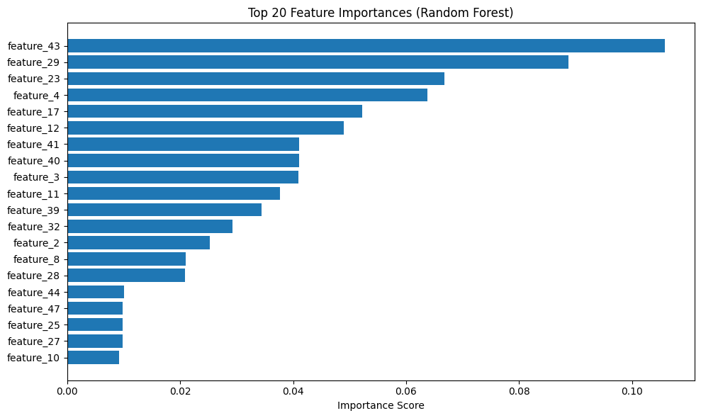
Step 3: Select Top Features
# Keep top K features (e.g., top 20)
K = 20
top_features = importance_df.head(K)['feature'].tolist()

print(f"\nSelected {K} features:")
print(top_features)

# Create reduced dataset
X_reduced = df[top_features]
print(f"\nReduced dataset shape: {X_reduced.shape}")
Selected 20 features:
['feature_43', 'feature_29', 'feature_23', 'feature_4', 'feature_17', 'feature_12', 'feature_41', 'feature_40', 'feature_3', 'feature_11', 'feature_39', 'feature_32', 'feature_2', 'feature_8', 'feature_28', 'feature_44', 'feature_47', 'feature_25', 'feature_27', 'feature_10']

Reduced dataset shape: (1000, 20)
Result: You’ve gone from 50 features to 20 features, keeping only the most informative ones.
Using XGBoost for Feature Importance
When to use: For regression tasks or when you want gradient boosting’s importance scores (often more accurate than Random Forest).
import xgboost as xgb
from sklearn.datasets import make_regression

# Generate regression dataset
X, y = make_regression(
    n_samples=1000,
    n_features=50,
    n_informative=15,
    random_state=42
)

feature_names = [f'feature_{i}' for i in range(50)]

# Train XGBoost
xgb_model = xgb.XGBRegressor(
    n_estimators=100,
    max_depth=6,
    learning_rate=0.1,
    random_state=42
)

xgb_model.fit(X, y)

# Get importances (default: weight = number of times feature is used for split)
importances = xgb_model.feature_importances_

# Create DataFrame
importance_df = pd.DataFrame({
    'feature': feature_names,
    'importance': importances
}).sort_values('importance', ascending=False)

print("Top 15 features (XGBoost):")
print(importance_df.head(15))
XGBoost importance types:
weight: Number of times feature is used in a split (default)gain: Average gain when feature is usedcover: Average coverage (samples affected) when feature is used
# Get different importance types
importance_gain = xgb_model.get_booster().get_score(importance_type='gain')
importance_cover = xgb_model.get_booster().get_score(importance_type='cover')
Complete Feature Selection Workflow
Production-ready workflow for selecting features from high-dimensional data:
from sklearn.model_selection import train_test_split
from sklearn.preprocessing import StandardScaler

def select_features_with_rf(df, target_col, n_features=50, random_state=42):
    """
    Select top N features using Random Forest importance.

    Args:
        df: DataFrame with features and target
        target_col: Name of target column
        n_features: Number of features to select
        random_state: Random seed

    Returns:
        selected_features: List of selected feature names
        importance_df: DataFrame with all features and their importance scores
    """
    # Separate features and target
    feature_cols = [col for col in df.columns if col != target_col]
    X = df[feature_cols]
    y = df[target_col]

    # Split data (only train on training set to avoid leakage)
    X_train, X_test, y_train, y_test = train_test_split(
        X, y, test_size=0.2, random_state=random_state
    )

    # Train Random Forest on training set only
    rf = RandomForestClassifier(
        n_estimators=100,
        max_depth=10,
        random_state=random_state,
        n_jobs=-1  # Use all CPU cores
    )

    rf.fit(X_train, y_train)

    # Get importances
    importance_df = pd.DataFrame({
        'feature': feature_cols,
        'importance': rf.feature_importances_
    }).sort_values('importance', ascending=False)

    # Select top N
    selected_features = importance_df.head(n_features)['feature'].tolist()

    # Report
    print(f"Selected {n_features} features from {len(feature_cols)} total")
    print(f"Top 10: {selected_features[:10]}")

    # Validation: Check if selected features actually improve model
    rf_reduced = RandomForestClassifier(
        n_estimators=100,
        max_depth=10,
        random_state=random_state
    )

    # Train on full features
    rf.fit(X_train, y_train)
    score_full = rf.score(X_test, y_test)

    # Train on selected features only
    rf_reduced.fit(X_train[selected_features], y_train)
    score_reduced = rf_reduced.score(X_test[selected_features], y_test)

    print(f"\nValidation accuracy:")
    print(f"  All features ({len(feature_cols)}): {score_full:.3f}")
    print(f"  Selected features ({n_features}): {score_reduced:.3f}")
    print(f"  Difference: {score_reduced - score_full:.3f}")

    return selected_features, importance_df

# Example usage
# selected_features, importance_df = select_features_with_rf(
#     df, target_col='label', n_features=50
# )
Interpreting Importance Scores
What Importance Tells You
High importance (e.g., > 0.05):
Feature is frequently used for splits
Feature creates pure separations between classes
Action: Keep this feature
Medium importance (e.g., 0.01 - 0.05):
Feature is somewhat useful
May be redundant with other features
Action: Keep if you have enough data; drop if overfitting
Low importance (e.g., < 0.01):
Feature rarely used or creates poor splits
Likely noise or highly correlated with other features
Action: Drop this feature
Pitfalls and Limitations
1. Biased toward high-cardinality features
Features with many unique values (e.g., user IDs) get inflated importance scores
Solution: Use permutation importance or validate with domain knowledge
2. Correlated features
If two features are correlated, only one may show high importance
The other appears unimportant even though it contains similar information
Solution: Manually inspect correlations and keep at most one from each correlated group
# Check correlations
corr_matrix = df[selected_features].corr().abs()
# Find pairs with correlation > 0.9
high_corr_pairs = []
for i in range(len(corr_matrix.columns)):
    for j in range(i+1, len(corr_matrix.columns)):
        if corr_matrix.iloc[i, j] > 0.9:
            high_corr_pairs.append((corr_matrix.columns[i], corr_matrix.columns[j]))

print(f"Highly correlated feature pairs: {high_corr_pairs}")
3. Doesn’t detect interactions
Individual features may be unimportant, but their interaction is critical
Example:
feature_Aandfeature_Balone are weak, butfeature_A * feature_Bis strongSolution: Manually engineer interaction features before computing importance
Best Practices
1. Always Use Training Data Only
Wrong (causes leakage):
# Fit on entire dataset
rf.fit(X, y)
selected_features = get_top_features(rf)
Right (no leakage):
# Split first
X_train, X_test, y_train, y_test = train_test_split(X, y)
# Fit only on training data
rf.fit(X_train, y_train)
selected_features = get_top_features(rf)
2. Validate Feature Selection
After selecting features, train a new model and verify performance doesn’t degrade:
# Full features
model_full.fit(X_train, y_train)
score_full = model_full.score(X_test, y_test)

# Reduced features
model_reduced.fit(X_train[selected_features], y_train)
score_reduced = model_reduced.score(X_test[selected_features], y_test)

# Should be close (within 2-3%)
assert score_reduced >= score_full - 0.03, "Too much performance loss!"
3. Use Multiple Methods
Don’t rely on a single importance metric. Compare:
Random Forest Gini importance
XGBoost gain importance
Permutation importance
Domain expert judgment
Features that rank high across multiple methods are reliably important.
4. Set a Threshold
Instead of picking top K features, select all features above an importance threshold:
# Keep features with importance > 1% of total
threshold = importances.sum() * 0.01
selected = importance_df[importance_df['importance'] > threshold]
Example: OCSF Security Logs
Use case: You have OCSF security logs with 300+ fields. Which fields are most predictive of security incidents?
# Assume you have labeled data (0=normal, 1=anomaly)
# This might come from historical incidents, SOC analyst labels, etc.

import pandas as pd
from sklearn.ensemble import RandomForestClassifier

# Load OCSF data with labels
# df = pd.read_csv('ocsf_logs_labeled.csv')

# Example feature columns (after flattening nested JSON)
ocsf_features = [
    'severity_id', 'activity_id', 'status_id',
    'actor_user_uid', 'src_endpoint_ip_subnet',
    'dst_endpoint_port', 'http_request_http_method',
    'bytes_per_second', 'failed_login_count_1h',
    'unique_ip_count_24h', 'hour_of_day', 'day_of_week',
    # ... 288 more features
]

# Select top 50 features
selected_features, importance_df = select_features_with_rf(
    df,
    target_col='is_anomaly',
    n_features=50
)

# Top 10 features for security anomaly detection:
# 1. failed_login_count_1h (0.085) - Brute force indicator
# 2. bytes_per_second (0.072) - Data exfiltration
# 3. unique_ip_count_24h (0.068) - Account compromise
# 4. dst_endpoint_port (0.051) - Unusual ports
# 5. hour_of_day (0.047) - Off-hours activity
# ...

print("Top features for anomaly detection:")
print(importance_df.head(10))Interpretation:
failed_login_count_1hhas highest importance → Brute force attacks are a major anomaly typebytes_per_secondis second → Data exfiltration is detectabledst_endpoint_portmatters → Connections to unusual ports are suspicious
Action: Use these 50 features to train your TabularResNet embedding model instead of all 300 fields.
When NOT to Use Tree-Based Importance
Don’t use for:
Linear models: Use L1 regularization (Lasso) coefficients instead
Neural networks: Use gradient-based attribution methods (GradCAM, integrated gradients)
Very small datasets (< 100 samples): Importance scores are unreliable
Alternative methods:
SHAP values: More accurate but slower (10-100x slower)
Mutual information: Good for non-linear relationships
Forward/backward selection: Iteratively add/remove features and measure performance
Summary
What we covered:
How tree-based models measure feature importance (Gini, permutation)
Using Random Forest and XGBoost for feature selection
Complete workflow for production feature selection
Interpreting importance scores and avoiding pitfalls
Best practices (train-only, validation, multiple methods)
Key takeaway: Tree-based feature importance is a fast, effective way to reduce high-dimensional data (100+ features) to a manageable subset (20-50 features) before training complex models.
Next steps:
Apply this workflow to your own dataset
Compare importance across Random Forest, XGBoost, and permutation methods
Validate that reduced features maintain model performance
Use selected features for downstream tasks (embeddings, classification, etc.)