The Hidden Power of Latent Factors - [DRAFT]

Why reducing dimensions can make models more powerful

The Counterintuitive Insight¶

Here’s a puzzle: You have a massive dataset with hundreds or thousands of dimensions. Your first instinct might be to preserve all that information—surely more dimensions mean more expressive power?

But across wildly different domains of machine learning, from recommendation systems to language models, we keep seeing the same pattern: Projecting high-dimensional data into lower-dimensional spaces makes models work better.

This isn’t just about computational efficiency (though that helps). It’s about forcing models to discover the essential structure hidden in the data.

In this post, we’ll explore this principle through two seemingly unrelated examples:

Alternating Least Squares (ALS) for movie recommendations
Multi-Head Attention in transformers

By the end, you’ll understand why “less is more” when it comes to dimensions.

import logging
import warnings

logging.getLogger("matplotlib.font_manager").setLevel(logging.ERROR)

import numpy as np
import matplotlib.pyplot as plt
import matplotlib.patches as mpatches
from matplotlib.patches import FancyBboxPatch, FancyArrowPatch, Rectangle
import torch

# Configure matplotlib
plt.rcParams['figure.facecolor'] = 'white'
plt.rcParams['axes.facecolor'] = 'white'
# Note: LaTeX rendering disabled to avoid build issues
# plt.rc('text', usetex=True)
# plt.rc('font', family='serif')

Part 1: The Core Principle¶

What Are Latent Factors?¶

Latent factors are hidden dimensions that capture the underlying patterns in data. They’re called “latent” (hidden) because:

They aren’t directly observed in the raw data
They’re learned automatically by algorithms
They often correspond to meaningful concepts, even though we never explicitly defined them

Think of them as the “real reasons” behind what we observe.

The Dimensionality Reduction Paradox¶

Consider a dataset with 1000 features. If we project it into just 50 dimensions, we’re throwing away 95% of the information, right?

Not quite. Here’s what actually happens:

fig, (ax1, ax2) = plt.subplots(1, 2, figsize=(14, 6))

# Left: High-dimensional noise
np.random.seed(42)
n_points = 200
n_dims_high = 1000

# Generate data that mostly lies on a low-dimensional manifold + noise
true_signal = np.random.randn(n_points, 10)  # 10 real dimensions
noise = np.random.randn(n_points, n_dims_high - 10) * 0.1  # 990 noise dimensions
high_dim_data = np.concatenate([true_signal, noise], axis=1)

# Calculate variance explained by each dimension
variance_explained = np.var(high_dim_data, axis=0)
sorted_variance = np.sort(variance_explained)[::-1]
cumulative_variance = np.cumsum(sorted_variance) / np.sum(sorted_variance)

ax1.bar(range(50), sorted_variance[:50], color='steelblue', alpha=0.7)
ax1.set_xlabel('Dimension (sorted by variance)', fontsize=12)
ax1.set_ylabel('Variance', fontsize=12)
ax1.set_title('Most Dimensions Contain Noise', fontsize=14, fontweight='bold')
ax1.axvline(x=10, color='red', linestyle='--', linewidth=2, label='Signal cutoff')
ax1.legend(fontsize=10)
ax1.grid(True, alpha=0.3)

# Right: Cumulative variance explained
ax2.plot(range(1, 101), cumulative_variance[:100], linewidth=3, color='darkgreen')
ax2.axhline(y=0.95, color='red', linestyle='--', linewidth=2, label='95% variance')
ax2.axvline(x=15, color='red', linestyle='--', linewidth=2, alpha=0.5)
ax2.fill_between(range(1, 101), 0, cumulative_variance[:100], alpha=0.2, color='green')
ax2.set_xlabel('Number of Dimensions', fontsize=12)
ax2.set_ylabel('Cumulative Variance Explained', fontsize=12)
ax2.set_title('First Few Dimensions Capture Most Signal', fontsize=14, fontweight='bold')
ax2.legend(fontsize=10)
ax2.grid(True, alpha=0.3)
ax2.set_xlim(0, 100)
ax2.set_ylim(0, 1.05)

plt.tight_layout()
plt.show()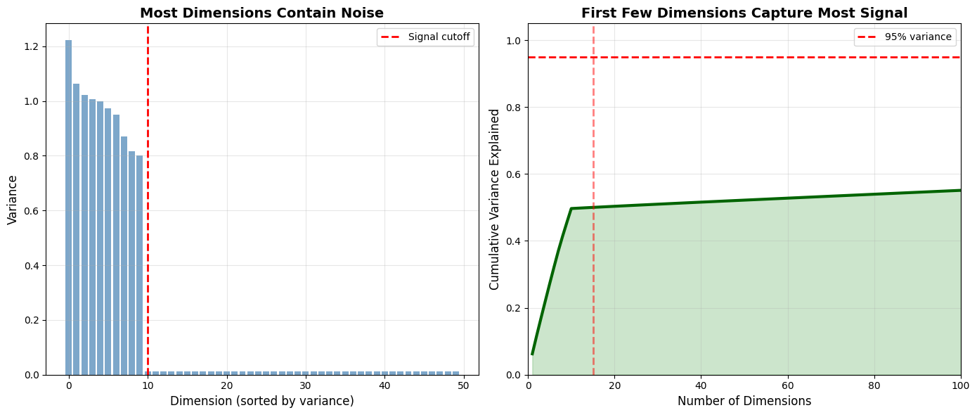

Key Insight: Real-world data rarely uses all available dimensions meaningfully. Most “dimensions” are just noise or redundant representations of the same underlying concepts.

By projecting to lower dimensions, we’re not losing information—we’re filtering out noise and forcing the model to learn what matters.

Part 2: Example 1 - ALS for Movie Recommendations¶

The Problem: Sparse Rating Matrices¶

Imagine Netflix’s rating matrix:

Rows: 200 million users
Columns: 50,000 movies
Total cells: 10 trillion possible ratings
Actual ratings: ~20 billion (0.2% filled)

This matrix is 99.8% empty. But hidden in those sparse ratings are patterns: some users love action movies, others prefer documentaries, some movies appeal to specific demographics.

The ALS Solution: Matrix Factorization¶

ALS decomposes this giant sparse matrix into two smaller dense matrices:

R_{m \times n} \approx U_{m \times k} \times M_{k \times n}^T

(1)

Where:

$R$ : User-item rating matrix (200M × 50K)
$U$ : User factors (200M × $k$ )
$M$ : Movie factors (50K × $k$ )
$k$ : Number of latent factors (typically 10-50)

fig = plt.figure(figsize=(16, 7))
ax = fig.add_subplot(111)
ax.axis('off')

# Dimensions
users, movies = 8, 10
factors = 3

# Rating matrix (left)
rating_x, rating_y = 0.5, 2
rating_w, rating_h = 3, 2.4

rect_rating = FancyBboxPatch(
    (rating_x, rating_y), rating_w, rating_h,
    boxstyle="round,pad=0.1",
    facecolor='#e3f2fd',
    edgecolor='#1976d2',
    linewidth=3
)
ax.add_patch(rect_rating)

# Add sparse pattern
np.random.seed(42)
sparse_mask = np.random.rand(users, movies) < 0.2
for i in range(users):
    for j in range(movies):
        if sparse_mask[i, j]:
            x = rating_x + 0.3 + (j * rating_w / movies)
            y = rating_y + 0.3 + (i * rating_h / users)
            ax.plot(x, y, 'o', color='#ff6f00', markersize=8, alpha=0.7)

ax.text(rating_x + rating_w/2, rating_y + rating_h + 0.4,
        r'\textbf{Rating Matrix } $R$',
        ha='center', fontsize=16, weight='bold')
ax.text(rating_x + rating_w/2, rating_y + rating_h + 0.1,
        r'$200M \times 50K$ (99.8\% empty)',
        ha='center', fontsize=12, style='italic', color='#555')

# Approximately equals sign
ax.text(5, rating_y + rating_h/2, r'$\approx$',
        ha='center', va='center', fontsize=50, weight='bold')

# User factors (right top)
user_x, user_y = 6.5, 3.2
user_w, user_h = 1.5, 2.4

rect_user = FancyBboxPatch(
    (user_x, user_y), user_w, user_h,
    boxstyle="round,pad=0.1",
    facecolor='#fff3e0',
    edgecolor='#f57c00',
    linewidth=3
)
ax.add_patch(rect_user)

ax.text(user_x + user_w/2, user_y + user_h + 0.4,
        r'\textbf{User Factors } $U$',
        ha='center', fontsize=14, weight='bold')
ax.text(user_x + user_w/2, user_y + user_h + 0.1,
        r'$200M \times k$',
        ha='center', fontsize=11, style='italic', color='#555')

# Multiplication sign
ax.text(8.7, rating_y + rating_h/2, r'$\times$',
        ha='center', va='center', fontsize=40, weight='bold')

# Movie factors (right bottom)
movie_x, movie_y = 9.5, 2
movie_w, movie_h = 2.4, 1.5

rect_movie = FancyBboxPatch(
    (movie_x, movie_y), movie_w, movie_h,
    boxstyle="round,pad=0.1",
    facecolor='#e8f5e9',
    edgecolor='#388e3c',
    linewidth=3
)
ax.add_patch(rect_movie)

ax.text(movie_x + movie_w/2, movie_y + movie_h + 0.4,
        r'\textbf{Movie Factors } $M^T$',
        ha='center', fontsize=14, weight='bold')
ax.text(movie_x + movie_w/2, movie_y + movie_h + 0.1,
        r'$k \times 50K$',
        ha='center', fontsize=11, style='italic', color='#555')

# Explanatory box
explanation = (
    r"\textbf{The Compression:}"
    "\n"
    r"Instead of storing $10$ trillion sparse values,"
    "\n"
    r"we store $10$ billion dense values ($k=50$)"
    "\n\n"
    r"\textbf{The Magic:}"
    "\n"
    r"$k$ latent factors capture hidden preferences"
    "\n"
    r"(genre, era, style, mood, actors, ...)"
)

ax.text(13.5, 3, explanation,
        fontsize=11, ha='left', va='center',
        bbox=dict(boxstyle='round,pad=0.8',
                 facecolor='#fffde7',
                 edgecolor='#f57f17',
                 linewidth=2))

ax.set_xlim(0, 16)
ax.set_ylim(0, 7)

plt.tight_layout()
plt.show()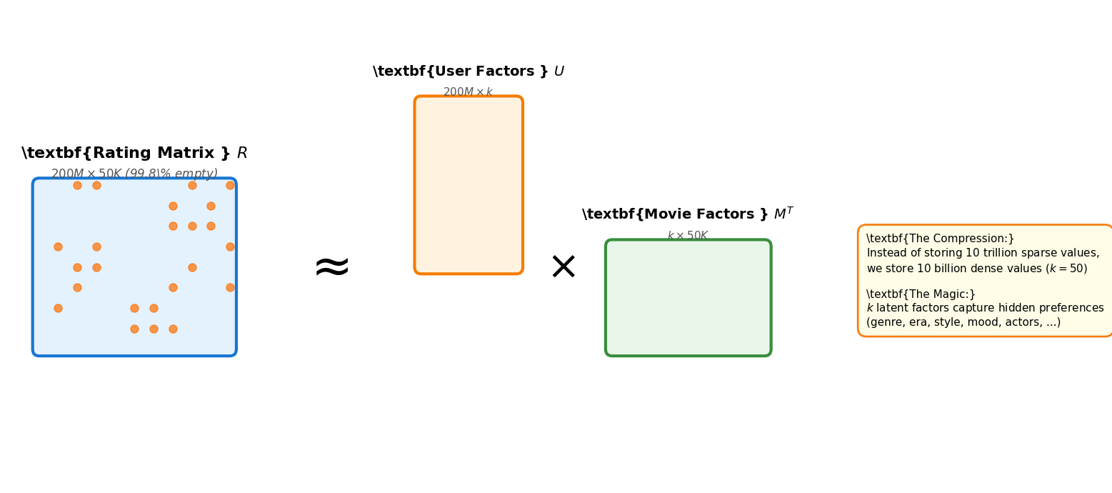

What Do These Latent Factors Mean?¶

The algorithm discovers patterns automatically. After training, we might find:

Factor 1: Action/adventure preference (high for Mad Max, low for Pride and Prejudice)
Factor 2: Serious vs. lighthearted (high for documentaries, low for comedies)
Factor 3: Classic vs. modern (high for Casablanca, low for recent releases)

Crucially: We never told the model “this is an action movie” or “this user likes comedies.” It learned these patterns from ratings alone.

Why Fewer Dimensions Work Better¶

# Simulate RMSE vs number of factors
factors_range = [2, 5, 10, 20, 50, 100, 200, 500]
train_rmse = [1.2, 0.95, 0.85, 0.82, 0.81, 0.80, 0.79, 0.78]
test_rmse = [1.25, 0.98, 0.88, 0.84, 0.83, 0.85, 0.90, 1.02]

fig, ax = plt.subplots(figsize=(10, 6))

ax.plot(factors_range, train_rmse, 'o-', linewidth=3, markersize=8,
        label='Training RMSE', color='#1976d2')
ax.plot(factors_range, test_rmse, 's-', linewidth=3, markersize=8,
        label='Test RMSE', color='#d32f2f')

# Mark optimal point
optimal_idx = np.argmin(test_rmse)
ax.axvline(x=factors_range[optimal_idx], color='green', linestyle='--',
           linewidth=2, alpha=0.7, label=f'Optimal ($k={factors_range[optimal_idx]}$)')
ax.plot(factors_range[optimal_idx], test_rmse[optimal_idx],
        'g*', markersize=20, label='Best generalization')

ax.set_xlabel(r'Number of Latent Factors ($k$)', fontsize=13)
ax.set_ylabel(r'RMSE (lower is better)', fontsize=13)
ax.set_title(r'\textbf{The Sweet Spot: Not Too Few, Not Too Many}', fontsize=15)
ax.set_xscale('log')
ax.grid(True, alpha=0.3)
ax.legend(fontsize=11, loc='upper right')

# Annotate regions
ax.annotate('Underfitting\n(too simple)', xy=(5, 0.95), xytext=(3, 1.1),
            fontsize=11, ha='center', color='#d32f2f',
            arrowprops=dict(arrowstyle='->', color='#d32f2f', lw=2))
ax.annotate('Overfitting\n(memorizing noise)', xy=(500, 1.02), xytext=(300, 1.15),
            fontsize=11, ha='center', color='#d32f2f',
            arrowprops=dict(arrowstyle='->', color='#d32f2f', lw=2))

plt.tight_layout()
plt.show()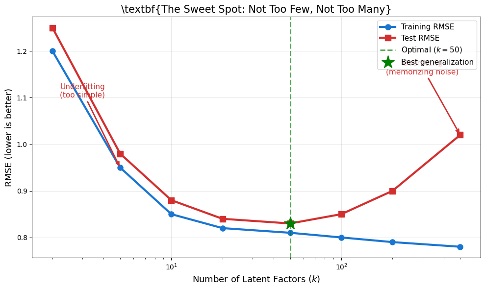

Why this happens:

Too few factors ( $k=2$ ): Can’t capture the complexity of human taste
Too many factors ( $k=500$ ): Starts memorizing individual ratings instead of learning patterns
Just right ( $k=20-50$ ): Captures real patterns while ignoring noise

Part 3: Example 2 - Multi-Head Attention in Transformers¶

The Problem: Understanding Language¶

Consider the sentence:

“The bank by the river was steep, but the bank downtown was closed.”

The word “bank” means different things based on context. A single 512-dimensional embedding must somehow encode:

Syntactic role (noun)
Semantic meaning (financial institution OR riverbank)
Relationships (to “river” vs. “downtown”)

The Multi-Head Solution: Parallel Subspaces¶

Instead of using one 512-dimensional attention mechanism, transformers use 8 parallel 64-dimensional mechanisms (called “heads”).

d_{model} = 512 \Rightarrow 8 \text{ heads} \times 64 \text{ dimensions each}

(2)

fig = plt.figure(figsize=(16, 8))
ax = fig.add_subplot(111)
ax.axis('off')

# Input embedding
input_x, input_y = 0.5, 1.5
input_w, input_h = 2, 6

rect_input = Rectangle((input_x, input_y), input_w, input_h,
                        facecolor='none', edgecolor='black', linewidth=3)
ax.add_patch(rect_input)

# Fill with colorful segments
num_segments = 20
colors = plt.cm.tab20.colors
for i in range(num_segments):
    seg_h = input_h / num_segments
    rect_seg = Rectangle((input_x, input_y + i*seg_h), input_w, seg_h,
                         facecolor=colors[i % len(colors)], alpha=0.7, edgecolor='none')
    ax.add_patch(rect_seg)

ax.text(input_x + input_w/2, input_y - 0.5,
        r'\textbf{Input Embedding}',
        ha='center', fontsize=14, weight='bold')
ax.text(input_x + input_w/2, input_y - 0.8,
        r'$d_{model} = 512$ dimensions',
        ha='center', fontsize=11, style='italic')
ax.text(input_x + input_w/2, input_y - 1.1,
        r'(mixed: syntax + semantics + context)',
        ha='center', fontsize=10, color='#555')

# Arrow and projection
ax.text(4.5, 4.5, "Linear Projection →",
        ha='center', va='center', fontsize=14)

# Output heads
head_x = 7
head_spacing = 1.2
head_w = 1.2
head_h = 1
colors_heads = ['#ffcdd2', '#f8bbd0', '#e1bee7', '#d1c4e9',
                '#c5cae9', '#bbdefb', '#b3e5fc', '#b2dfdb']
head_labels = ['Syntax', 'Coreference', 'Semantics', 'Position',
               'Entities', 'Sentiment', 'Tense', 'Dependencies']

for i in range(8):
    y_pos = 1.2 + i * head_spacing

    # Head box
    rect_head = FancyBboxPatch(
        (head_x, y_pos), head_w, head_h,
        boxstyle="round,pad=0.05",
        facecolor=colors_heads[i],
        edgecolor='black',
        linewidth=2
    )
    ax.add_patch(rect_head)

    # Head label
    ax.text(head_x + head_w/2, y_pos + head_h/2,
            f'Head {i+1}',
            ha='center', va='center', fontsize=10, weight='bold')

    # Dimension label
    ax.text(head_x + head_w + 0.1, y_pos + head_h/2,
            f'{head_labels[i]}\n($d_k=64$)',
            ha='left', va='center', fontsize=9)

    # Arrow from input to head
    arrow = FancyArrowPatch(
        (input_x + input_w, input_y + input_h/2),
        (head_x - 0.1, y_pos + head_h/2),
        arrowstyle='-|>',
        connectionstyle=f'arc3,rad={0.3*(i-3.5)/3.5}',
        color=colors_heads[i],
        linewidth=2,
        alpha=0.6,
        zorder=1
    )
    ax.add_patch(arrow)

# Explanation box
explanation = (
    r"\textbf{Key Insight:}"
    "\n\n"
    r"Each head specializes by having"
    "\n"
    r"\textit{fewer} dimensions ($64$ vs $512$)"
    "\n\n"
    r"Constraint $\Rightarrow$ Forces selectivity"
    "\n\n"
    r"8 specialists $>$ 1 generalist"
)

ax.text(12.5, 4.5, explanation,
        fontsize=11, ha='left', va='center',
        bbox=dict(boxstyle='round,pad=0.8',
                 facecolor='#fff9c4',
                 edgecolor='#f57f17',
                 linewidth=2))

ax.set_xlim(0, 15)
ax.set_ylim(0, 11)

plt.tight_layout()
plt.show()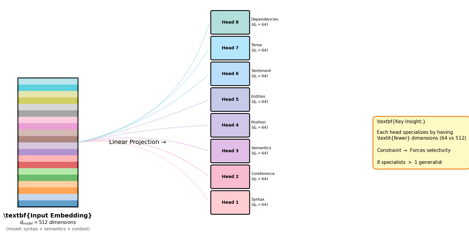

What Do These Heads Learn?¶

Research analyzing trained transformers found heads specializing in:

Syntactic heads: Track subject-verb agreement, noun-adjective relationships
Positional heads: Attend to previous/next tokens
Semantic heads: Link pronouns to their referents (“it” → “bank”)
Rare word heads: Focus on low-frequency vocabulary

Again, these roles emerge from training—we never explicitly told heads what to focus on.

Why Multiple Lower-Dimensional Heads?¶

Let’s compare three approaches:

fig, axes = plt.subplots(1, 3, figsize=(16, 5))

approaches = [
    {
        'title': r'\textbf{Approach A: Single Full-Dim Head}',
        'config': '1 head × 512 dims',
        'params': '512 × 512 = 262K params (per Q/K/V)',
        'cost': 'Compute: $O(n^2 d)$ with $d=512$',
        'quality': 'Learns averaged attention patterns',
        'color': '#ef5350'
    },
    {
        'title': r'\textbf{Approach B: 8 Full-Dim Heads}',
        'config': '8 heads × 512 dims each',
        'params': '8 × (512 × 512) = 2.1M params',
        'cost': 'Compute: $8 \\times O(n^2 d)$ (expensive!)',
        'quality': 'Might learn redundant patterns',
        'color': '#ff9800'
    },
    {
        'title': r'\textbf{Approach C: 8 Split-Dim Heads}',
        'config': '8 heads × 64 dims each',
        'params': '8 × (512 × 64) = 262K params (same as A!)',
        'cost': 'Compute: $O(n^2 d)$ with $d=64 \\times 8$',
        'quality': 'Learns specialized patterns ✓',
        'color': '#66bb6a'
    }
]

for ax, approach in zip(axes, approaches):
    ax.set_xlim(0, 10)
    ax.set_ylim(0, 10)
    ax.axis('off')

    # Title
    ax.text(5, 9, approach['title'], ha='center', fontsize=13, weight='bold')

    # Visual representation
    if approach['config'].startswith('1 head'):
        # Single large box
        rect = Rectangle((2, 4), 6, 3, facecolor=approach['color'],
                        edgecolor='black', linewidth=2, alpha=0.7)
        ax.add_patch(rect)
        ax.text(5, 5.5, '512-dim', ha='center', va='center',
               fontsize=12, weight='bold', color='white')
    elif approach['config'].startswith('8 heads × 512'):
        # 8 large boxes stacked
        for i in range(4):
            rect = Rectangle((1, 4 + i*0.6), 3.5, 0.5,
                           facecolor=approach['color'],
                           edgecolor='black', linewidth=1, alpha=0.7)
            ax.add_patch(rect)
        ax.text(2.75, 6.5, '...', ha='center', fontsize=16, weight='bold')
        ax.text(7, 5.5, '512-dim\neach', ha='center', va='center', fontsize=10)
    else:
        # 8 small boxes
        for i in range(4):
            rect = Rectangle((2, 4 + i*0.8), 2, 0.6,
                           facecolor=approach['color'],
                           edgecolor='black', linewidth=1, alpha=0.7)
            ax.add_patch(rect)
        ax.text(4, 6.8, '...', ha='center', fontsize=16, weight='bold')
        ax.text(7, 5.5, '64-dim\neach', ha='center', va='center', fontsize=10)

    # Details
    details = f"{approach['params']}\n{approach['cost']}\n\n{approach['quality']}"
    ax.text(5, 2, details, ha='center', va='center', fontsize=9,
           bbox=dict(boxstyle='round,pad=0.5', facecolor='white',
                    edgecolor=approach['color'], linewidth=2))

plt.tight_layout()
plt.show()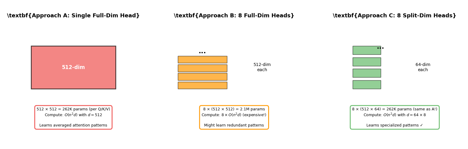

Approach C wins because:

Same parameter count as single-head (no extra memory)
Similar computational cost (parallelizes well on GPUs)
Better quality through specialization

Part 4: The Deep Connection¶

Both techniques follow the same fundamental pattern:

fig, ax = plt.subplots(figsize=(14, 10))
ax.axis('off')
ax.set_xlim(0, 14)
ax.set_ylim(0, 12)

# Title
ax.text(7, 11, r'\textbf{The Latent Factor Pattern}',
        ha='center', fontsize=18, weight='bold')

# Column headers
ax.text(3.5, 9.5, r'\textbf{ALS (Recommendations)}',
        ha='center', fontsize=14, weight='bold', color='#f57c00')
ax.text(10.5, 9.5, r'\textbf{Multi-Head Attention (Language)}',
        ha='center', fontsize=14, weight='bold', color='#1976d2')

# Row 1: High-dimensional input
y_pos = 8.5
ax.text(0.5, y_pos, r'\textbf{1. Start}', ha='left', fontsize=12, weight='bold')

ax.text(3.5, y_pos,
        r'Sparse rating matrix\n$200M \times 50K$ (99.8\% empty)',
        ha='center', fontsize=10,
        bbox=dict(boxstyle='round,pad=0.5', facecolor='#fff3e0', edgecolor='#f57c00', linewidth=2))

ax.text(10.5, y_pos,
        r'Token embedding\n$512$ dimensions (mixed info)',
        ha='center', fontsize=10,
        bbox=dict(boxstyle='round,pad=0.5', facecolor='#e3f2fd', edgecolor='#1976d2', linewidth=2))

# Row 2: Decomposition
y_pos = 6.5
ax.text(0.5, y_pos, r'\textbf{2. Decompose}', ha='left', fontsize=12, weight='bold')

ax.text(3.5, y_pos,
        r'Factor into $k$ latent dimensions\n$U_{m \times k} \times M_{k \times n}^T$ with $k \approx 20$',
        ha='center', fontsize=10,
        bbox=dict(boxstyle='round,pad=0.5', facecolor='#fff3e0', edgecolor='#f57c00', linewidth=2))

ax.text(10.5, y_pos,
        r'Split into $h$ attention heads\n$h \times (d_{model}/h)$ with $h=8, d_k=64$',
        ha='center', fontsize=10,
        bbox=dict(boxstyle='round,pad=0.5', facecolor='#e3f2fd', edgecolor='#1976d2', linewidth=2))

# Row 3: What gets learned
y_pos = 4.5
ax.text(0.5, y_pos, r'\textbf{3. Discover}', ha='left', fontsize=12, weight='bold')

ax.text(3.5, y_pos,
        r'Hidden preferences:\n• Action vs. drama\n• Serious vs. lighthearted\n• Classic vs. modern',
        ha='center', fontsize=9,
        bbox=dict(boxstyle='round,pad=0.5', facecolor='#fff3e0', edgecolor='#f57c00', linewidth=2))

ax.text(10.5, y_pos,
        r'Specialized patterns:\n• Syntax \& grammar\n• Coreference resolution\n• Semantic relationships',
        ha='center', fontsize=9,
        bbox=dict(boxstyle='round,pad=0.5', facecolor='#e3f2fd', edgecolor='#1976d2', linewidth=2))

# Row 4: Why it works
y_pos = 2.5
ax.text(0.5, y_pos, r'\textbf{4. Why}', ha='left', fontsize=12, weight='bold')

ax.text(3.5, y_pos,
        r'Low rank $\Rightarrow$ forces generalization\nFilters noise, learns patterns',
        ha='center', fontsize=9,
        bbox=dict(boxstyle='round,pad=0.5', facecolor='#fff3e0', edgecolor='#f57c00', linewidth=2))

ax.text(10.5, y_pos,
        r'Low dim per head $\Rightarrow$ forces specialization\nEach head focuses on one aspect',
        ha='center', fontsize=9,
        bbox=dict(boxstyle='round,pad=0.5', facecolor='#e3f2fd', edgecolor='#1976d2', linewidth=2))

# Central insight box
insight = (
    r"\textbf{The Shared Principle:}"
    "\n\n"
    r"Reducing dimensions \textit{constrains} the model"
    "\n\n"
    r"Constraints force discovery of \textit{essential structure}"
    "\n\n"
    r"Essential structure $=$ what actually matters"
)

ax.text(7, 0.5, insight,
        ha='center', va='center', fontsize=11,
        bbox=dict(boxstyle='round,pad=0.8', facecolor='#f1f8e9',
                 edgecolor='#558b2f', linewidth=3))

plt.tight_layout()
plt.show()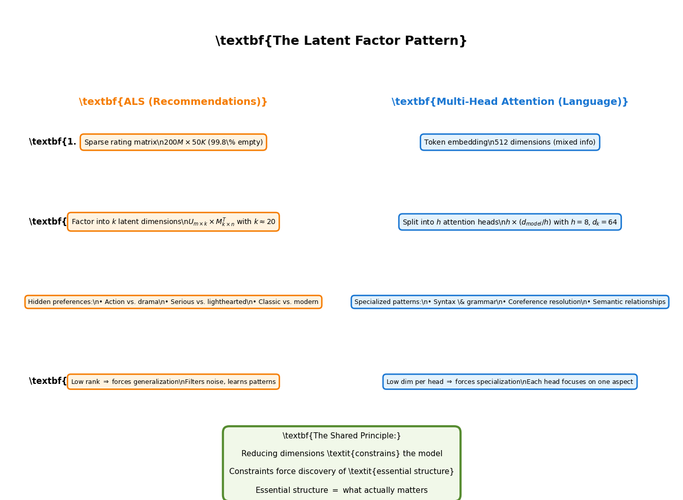

The Mathematical Connection¶

Both use the same core trick: low-rank approximation.

ALS: Approximate rank- $r$ matrix with rank- $k$ factorization ( $k \ll r$ )

R \approx UV^T

(3)

Multi-Head Attention: Instead of one $d$ -dimensional space, use $h$ subspaces of dimension $d/h$

\text{MultiHead}(Q,K,V) = \text{Concat}(\text{head}_1, \ldots, \text{head}_h) W^O

(4)

Both work because:

Real patterns are low-dimensional: Human preferences and language structure don’t need millions of dimensions
Constraints prevent overfitting: Fewer dimensions = can’t memorize noise
Specialization emerges naturally: Multiple subspaces learn different aspects

Part 5: When to Use This Pattern¶

The Decision Framework¶

Use dimensionality reduction when:

✅ Data has hidden structure: Relationships between features exist but aren’t explicit ✅ High sparsity: Most feature combinations never occur ✅ Need generalization: Want to predict unseen combinations ✅ Interpretability matters: Want to understand what the model learned

Avoid when:

❌ Every dimension is meaningful: No redundancy in features ❌ Dense data: All combinations are observed ❌ Exact reconstruction needed: Can’t afford any approximation error

Practical Guidelines¶

For recommendation systems:

Start with $k = 10$ , increase until test error plateaus
Typical range: 10-50 factors for most datasets
More factors needed for large catalogs (millions of items)

For transformers:

Standard: 8-16 heads with $d_k = d_{model}/h$
Smaller models (BERT-base): 12 heads, $d_k = 64$
Larger models (GPT-3): 96 heads, $d_k = 128$
Keep $d_k$ between 32-128 for best results

Summary¶

The latent factor principle appears across machine learning because it captures a fundamental truth: real-world complexity often has simple underlying structure.

Key Takeaways¶

Reducing dimensions ≠ losing information when most “dimensions” are noise or redundancy
Constraints enable discovery: Forcing models into lower dimensions makes them learn what truly matters
Specialization through separation: Multiple small subspaces often outperform one large space
Patterns emerge, not assigned: In both ALS and multi-head attention, roles are learned through training, not programmed
Universal applicability: This pattern works for recommendations, language, images, graphs, and more

The Deeper Lesson¶

When you encounter a high-dimensional problem, your first instinct might be to preserve all dimensions. But often, the right move is counterintuitive: compress first, then learn.

The magic happens in the compression. By forcing information through a bottleneck, you filter out noise and surface the essential patterns that actually matter.