L04 - Multi-Head Attention: The Committee of Experts

Why one brain is good, but eight brains are better.

In L03 - Self-Attention, we built the “Search Engine” of the Transformer. We learned how the word “it” can look up the word “animal” to resolve ambiguity.

But there is a limitation. A single self-attention layer acts like a single pair of eyes. It can focus on one aspect of the sentence at a time. Consider the sentence:

The chicken didn’t cross the road because it was too wide.

To understand this fully, the model needs to do two things simultaneously:

Syntactic Analysis: Link “it” to the subject “road” (because roads are wide).
Semantic Analysis: Understand that “wide” is a physical property preventing crossing.

If we only have one attention head, the model has to average these different relationships into a single vector. It muddies the waters.

Multi-Head Attention solves this by giving the model multiple “heads” (independent attention mechanisms) that run in parallel.

By the end of this post, you’ll understand:

The intuition of the “Committee of Experts.”
Why we project vectors into different Subspaces.
How to implement the tensor reshaping magic (view and transpose) in PyTorch.

import os
import logging
import warnings

logging.getLogger("matplotlib.font_manager").setLevel(logging.ERROR)

import torch
import torch.nn as nn
import matplotlib
import matplotlib.pyplot as plt
import numpy as np

plt.rcParams['figure.facecolor'] = 'white'
plt.rcParams['axes.facecolor'] = 'white'

torch.manual_seed(0)

Part 1: The Intuition (The Committee)¶

The Committee Metaphor¶

Think of the embedding dimension ( $d_{model} = 512$ ) as a massive report containing everything we know about a word.

If we ask a single person to read that report and summarize “grammar,” “tone,” “tense,” and “meaning” all at once, they might miss details.

Instead, we hire a Committee of 8 Experts:

Head 1 (The Linguist): Only looks for Subject-Verb agreement.
Head 2 (The Historian): Looks for past/present tense consistency.
Head 3 (The Translator): Looks for definitions and synonyms.
...

In the Transformer, we don’t just copy the input 8 times. We project the input into 8 different lower-dimensional spaces. This allows each head to specialize.

Visualizing Multi-Head Projection¶

Let’s visualize this head specialization. In the plot below:

The Input (Mixed Info): The large multi-colored bar represents the full word embedding ( $d=512$ ).
The Projection: We project this into 8 equal-sized subspaces ( $d_k = 64$ ).
The Result: Each head gets a vector that is 1/8th the size of the original, containing only the specific info it needs.

import matplotlib.pyplot as plt
import matplotlib.patches as patches
import numpy as np

def plot_multihead_projection_concept():
    fig, ax = plt.subplots(figsize=(14, 8)) # Increased size slightly
    ax.set_xlim(0, 14)
    ax.set_ylim(0, 9)
    ax.axis('off')

    # --- Configuration ---
    input_x = 1
    output_x = 10

    # Coordinates for the "Heads" (Outputs)
    # We show them essentially "stacking up" to equal the total concept,
    # but separated to show independence.
    y_positions = [7, 4.5, 2]
    colors = ['#FF9999', '#99FF99', '#9999FF']
    labels = ["Head 1\nGrammar", "Head 2\nTense", "Head 3\nMeaning"]

    # FONT SIZES
    font_title = 20
    font_label = 16
    font_math = 14
    font_annot = 14

    # --- 1. Draw Input Vector (The "General Report") ---
    height = 6
    width = 1.5
    base_y = 1.5

    # Container
    input_rect = patches.Rectangle((input_x, base_y), width, height, linewidth=3, edgecolor='black', facecolor='none', zorder=5)
    ax.add_patch(input_rect)

    # "Mixed Info" bands
    num_segments = 20
    seg_height = height / num_segments
    np.random.seed(42)
    segment_colors = plt.get_cmap('tab20').colors
    for i in range(num_segments):
        color = segment_colors[i % len(segment_colors)]
        rect = patches.Rectangle((input_x, base_y + i*seg_height), width, seg_height, facecolor=color, alpha=0.7, edgecolor='none')
        ax.add_patch(rect)

    # Label Input
    ax.text(input_x + width/2, base_y - 0.6, "Input Embedding\n($d_{model}=512$)", ha='center', va='top', fontweight='bold', fontsize=font_label)

    # --- 2. Draw The Projections (Arrows & Matrices) ---

    proj_start_x = input_x + width + 0.2
    proj_end_x = output_x - 0.2

    for i, (y_c, color, label) in enumerate(zip(y_positions, colors, labels)):
        # A. Arrow from Input Center to Head Center
        arrow = patches.FancyArrowPatch(
            (proj_start_x, base_y + height/2), (proj_end_x, y_c),
            arrowstyle='-|>,head_width=0.6,head_length=1.0',
            connectionstyle=f"arc3,rad={(i-1)*-0.15}",
            color=color, lw=4, zorder=2, alpha=0.8
        )
        ax.add_patch(arrow)

        # B. Matrix Box (The "Lens")
        mid_x = (proj_start_x + proj_end_x) / 2
        mid_y = (base_y + height/2 + y_c) / 2 + (i-1)*0.5 # Slight offset for visual separation

        # Matrix Label
        ax.text(mid_x, mid_y + 0.6, f"$W_{i}$", ha='center', va='center', color=color, fontweight='bold', fontsize=font_label, zorder=6)

        # C. Output Subspace Blocks
        # Make them look identical in size
        out_h = 1.8
        out_w = 1.5
        out_rect = patches.Rectangle((output_x, y_c - out_h/2), out_w, out_h, facecolor=color, edgecolor='black', lw=2, alpha=0.9)
        ax.add_patch(out_rect)

        # Label each head
        ax.text(output_x + out_w + 0.3, y_c, label, ha='left', va='center', fontsize=font_label, color='black')
        # Math label showing the split
        ax.text(output_x + out_w + 0.3, y_c - 0.6, "($d_k=64$)", ha='left', va='center', fontsize=font_math, color='#555')

    # --- 3. Final Annotations describing the Split ---

    # Title
    ax.text(7, 8.5, "Multi-Head Projection: Dividing the Work", ha='center', va='center', fontsize=font_title, fontweight='bold')

    # Explanation of the split
    ax.text(7, 0.5, "Total Dimensions (512) $\\div$ Heads (8) = 64 dims per Head",
            ha='center', va='center', fontsize=font_label, fontweight='bold',
            bbox=dict(facecolor='#f0f0f0', edgecolor='gray', boxstyle='round,pad=0.5'))

    plt.tight_layout()
    plt.show()

plot_multihead_projection_concept()

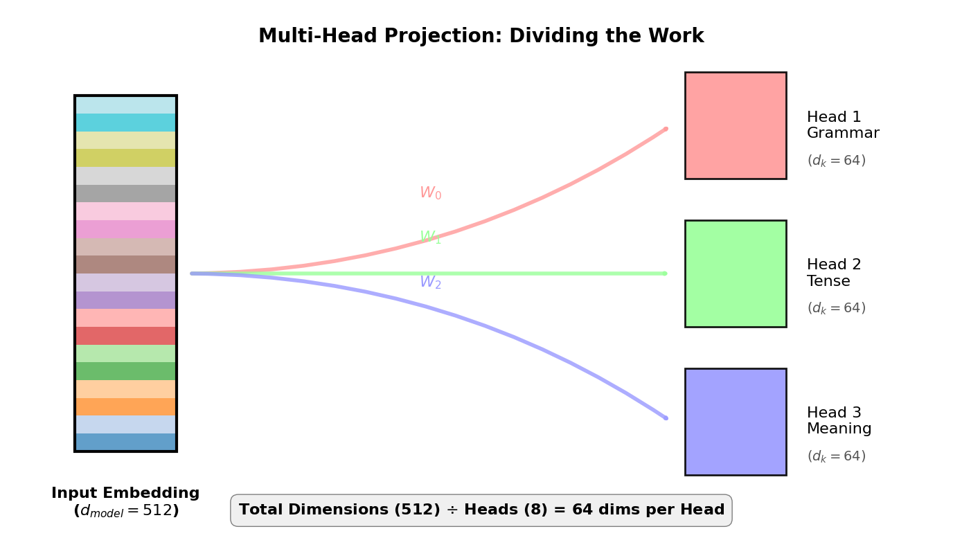
We draw 3 heads for readability—imagine 8 in the real model.

Parameter Implications: Why Reduced Dimensions?¶

Let’s look at the parameter implications of using reduced dimensions (64) per head instead of full dimensions (512):

# Parameter-count intuition: "full 512 per head" vs "reduced dims per head (8×64)"
d_model = 512
h = 8
d_k = d_model // h  # Each head gets 64 dimensions instead of 512

# Scenario A: Each head gets full 512-dim projections (wasteful)
# Would need 8 separate (512×512) matrices for EACH of Q, K, V (3 matrices total)
params_if_full = 3 * h * (d_model * d_model)  # 3 = Q, K, V

# Scenario B: Each head gets 64-dim projections (efficient)
# Need 8 × (512×64) matrices for EACH of Q, K, V (3 matrices total)
params_reduced = 3 * h * (d_model * d_k)  # 3 = Q, K, V

# Scenario C: One big matrix (actual implementation)
# Single (512×512) matrix for EACH of Q, K, V (3 matrices total)
# THEN reshape the 512-dim output into 8 heads × 64 dims (the "split" operation)
params_actual = 3 * (d_model * d_model)  # 3 = Q, K, V

print(f"d_model={d_model}, heads={h}, d_k={d_k}")

print("QKV parameters:")
print(f"  if full dims:     {params_if_full:,}")
print(f"  if reduced dims:  {params_reduced:,}")
print(f"  actual (1 big W): {params_actual:,}")
print(f"  reduced == actual? {params_reduced == params_actual}")
print()
print("Note: Scenario C has the SAME param count as single-head attention,")
print("but the difference is in the OUTPUT: we reshape it into 8 heads × 64 dims")

d_model=512, heads=8, d_k=64
QKV parameters:
  if full dims:     6,291,456
  if reduced dims:  786,432
  actual (1 big W): 786,432
  reduced == actual? True

Note: Scenario C has the SAME param count as single-head attention,
but the difference is in the OUTPUT: we reshape it into 8 heads × 64 dims

The code above shows that using reduced dimensions per head keeps parameters constant (786K vs 6.3M for full dimensions per head). But why do this instead of giving each head the full 512 dimensions?

Forced specialization. With only 64 dimensions, each head must be selective about what it captures, encouraging distinct patterns:

Head 1 might focus on syntax (subject-verb agreement)
Head 2 might focus on semantics (word meaning relationships)
Head 3 might focus on positional patterns (nearby vs distant dependencies)

Think of it like hiring specialists with limited notepads. If each expert had unlimited space, they might all write the same general report. But with only 64 dimensions, each head is forced to focus on what matters most to its specialized role.

How Heads Learn Their Roles¶

When we say “Head 1 (The Linguist)” we’re using a metaphor for intuition. In reality:

You only specify num_heads=8 in your code
The model learns what each head should focus on during training through backpropagation
The “roles” are emergent - they’re patterns discovered by gradient descent, not programmed by you
Descriptive, not prescriptive - Labels like “Linguist” are what researchers assign after analyzing what a trained model learned

You can’t tell the model “Head 1, you focus on grammar!” - it discovers its own patterns that minimize loss. Different training runs or datasets might result in different specializations.

Part 2: The Multi-Head Pipeline¶

Now that we understand the “why” (Specialization), let’s look at the “how” (The Pipeline).

The Multi-Head Attention mechanism isn’t a single black box; it is a specific sequence of operations. It allows the model to process information in parallel and then synthesize the results.

Let’s start with the big picture:

The 4-Step Process¶

Linear Projections (Mix, then Split): We don’t just use the raw input. We multiply the input $Q, K, V$ by specific weight matrices ( $W^Q_i, W^K_i, W^V_i$ ) for each head. This creates the specialized “subspaces” we saw in Part 1.
Independent Attention: Each head runs the standard Scaled Dot-Product Attention independently.
$\text{head}_i = \text{Attention}(QW_i^Q, KW_i^K, VW_i^V)$
(2)
Concatenation: Stitch the head outputs back together along the feature dimension.
Final Linear (Another Mix): Apply one last learned linear layer ( $W^O$ ) to blend the heads into a single unified vector.

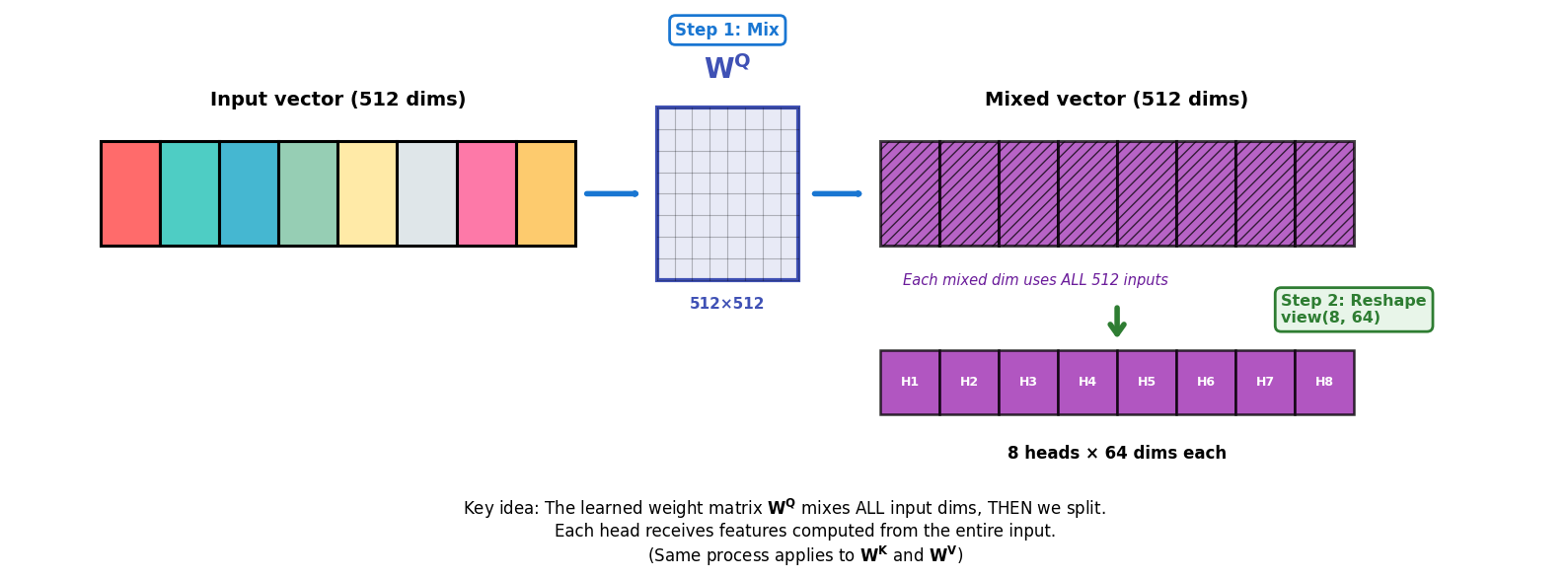
\text{MultiHead}(Q, K, V) = \text{Concat}(\text{head}_1, \dots, \text{head}_h)W^O

(3)

The Key Insight: Mix, Then Split¶

Now let’s zoom into Step 1, which is the operation most people misinterpret.

It’s tempting to think multi-head attention “just splits the 512 dims into 8 chunks.” That’s not what happens.

Instead, the split happens in two stages:

Mix (learned linear layer): We first apply a learned matrix ( $W^Q$ , $W^K$ , $W^V$ ). When you compute $Q = X \cdot W^Q$ , each of the 512 output dimensions is a weighted sum of ALL 512 input dimensions. This means the network can learn to combine any input features together before splitting into heads.
Note
These are the SAME $W^Q$ , $W^K$ , $W^V$ from L03! The projection matrices work identically - they’re still learned (512×512) matrices that mix input features. The only difference in L04 is what we do with the outputs: we reshape them into multiple heads instead of using them as-is.
Split (reshape/view): Only after that mix do we reshape the resulting 512-dimensional output into 8 heads × 64 dims.

Why does this matter? During training, the network can learn $W^Q$ such that:

Output dimensions 0-63 (Head 1’s slice) contain features useful for syntax
Output dimensions 64-127 (Head 2’s slice) contain features useful for semantics
And so on...

This is what enables head specialization—each head gets features specifically curated for its role, not just a random slice of the input.

Keep this invariant in mind: the split step only works when $D$ is divisible by $H$ so that $D = H \times d_k$ . If you change any of these values in the code, recompute d_k = D // H first.

# Concrete example: Prove that each output dimension mixes ALL input dimensions
torch.manual_seed(1)
D = 8  # Small example for clarity
x0 = torch.randn(D)           # One token vector [D]
W = torch.randn(D, D)         # Mix matrix (like W^Q, W^K, or W^V) [D×D]
q0 = x0 @ W                   # Matrix multiply: [D] @ [D×D] = [D]

print("=" * 60)
print("DEMONSTRATING THE MIX OPERATION")
print("=" * 60)
print(f"\nInput vector x0 (shape {x0.shape}):")
print(x0)
print(f"\nMix matrix W (shape {W.shape}):")
print(W)
print(f"\nOutput vector q0 = x0 @ W (shape {q0.shape}):")
print(q0)

# Proof: Pick any output dimension (let's use index 3) and show it depends on ALL inputs
output_idx = 3
print(f"\n--- Verifying q0[{output_idx}] uses ALL input dimensions ---")
print(f"q0[{output_idx}] = {q0[output_idx].item():.4f}")
print()

# Show the column of W that produces this output dimension
print(f"W[:, {output_idx}] (weights for output dimension {output_idx}):")
print(W[:, output_idx])
print()

# Manual computation: q0[j] = dot product of x0 with column j of W
manual = (x0 * W[:, output_idx]).sum()  # x0[0]*W[0,3] + x0[1]*W[1,3] + ... + x0[7]*W[7,3]
print(f"Manual calculation: sum of (x0[i] * W[i,{output_idx}]) for ALL i from 0 to {D-1}")
print(f"                  = {manual.item():.4f}")
print()
print(f"✓ Matches! This proves q0[{output_idx}] is a weighted combination of")
print(f"  ALL {D} input dimensions, not just one chunk.")
print("=" * 60)

============================================================
DEMONSTRATING THE MIX OPERATION
============================================================

Input vector x0 (shape torch.Size([8])):
tensor([ 0.6614,  0.2669,  0.0617,  0.6213, -0.4519, -0.1661, -1.5228,  0.3817])

Mix matrix W (shape torch.Size([8, 8])):
tensor([[-0.6970, -1.1608,  0.6995,  0.1991,  0.8657,  0.2444, -0.6629,  0.8073],
        [ 1.1017, -0.1759, -2.2456, -1.4465,  0.0612, -0.6177, -0.7981, -0.1316],
        [ 1.8793, -0.0721,  0.1578, -0.7735,  0.1991,  0.0457,  0.1530, -0.4757],
        [-0.1110,  0.2927, -0.1578, -0.0288,  2.3571, -1.0373,  1.5748, -0.6298],
        [-0.9274,  0.5451,  0.0663, -0.4370,  0.7626,  0.4415,  1.1651,  2.0154],
        [ 0.1374,  0.9386, -0.1860, -0.6446,  1.5392, -0.8696, -3.3312, -0.7479],
        [-0.0255, -1.0233, -0.5962, -1.0055, -0.2106, -0.0075,  1.6734,  0.0103],
        [-0.7040, -0.1853, -0.9962, -0.8313, -0.4610, -0.5601,  0.3956, -0.9823]])

Output vector q0 = x0 @ W (shape torch.Size([8])):
tensor([ 0.0465,  0.4481,  0.3035,  1.1985,  1.6100, -0.9023, -2.0339, -1.0991])

--- Verifying q0[3] uses ALL input dimensions ---
q0[3] = 1.1985

W[:, 3] (weights for output dimension 3):
tensor([ 0.1991, -1.4465, -0.7735, -0.0288, -0.4370, -0.6446, -1.0055, -0.8313])

Manual calculation: sum of (x0[i] * W[i,3]) for ALL i from 0 to 7
                  = 1.1985

✓ Matches! This proves q0[3] is a weighted combination of
  ALL 8 input dimensions, not just one chunk.
============================================================

Let’s visualize that “Mix → Split” distinction (shown for $\mathbf{W^Q}$ , but $W^K$ and $W^V$ work identically):

from matplotlib import pyplot as plt
import matplotlib.patches as patches
import matplotlib as mpl
import numpy as np

# mpl.rcParams['mathtext.fontset'] = 'stixsans'
# mpl.rcParams['mathtext.default'] = 'regular'


def plot_mix_then_split():
    """
    Visualizes the two-step process: Mix (Linear Transform) then Split (Reshape).
    Shows horizontal flow: Input -> W^Q -> Mixed -> Reshape -> Heads
    """
    fig, ax = plt.subplots(1, 1, figsize=(16, 6))
    ax.set_xlim(0, 17)
    ax.set_ylim(0, 6)
    ax.axis('off')

    # Geometry
    input_x, y = 1.0, 3.4
    input_width, input_height = 5.2, 1.15
    n_heads = 8
    seg_w = input_width / n_heads

    colors = [
        '#FF6B6B', '#4ECDC4', '#45B7D1', '#96CEB4',
        '#FFEAA7', '#DFE6E9', '#FD79A8', '#FDCB6E'
    ]

    # -------------------------
    # Input vector (512 dims)
    # -------------------------
    for i in range(n_heads):
        ax.add_patch(
            patches.Rectangle(
                (input_x + i * seg_w, y),
                seg_w, input_height,
                facecolor=colors[i],
                edgecolor='black',
                linewidth=2.2
            )
        )

    ax.text(
        input_x + input_width / 2, y + input_height + 0.35,
        "Input vector (512 dims)",
        ha='center', va='bottom',
        fontsize=14, fontweight='bold'
    )

    # -------------------------
    # W^Q matrix
    # -------------------------
    matrix_x = input_x + input_width + 0.9
    matrix_y = y + input_height / 2 - 0.95
    mw, mh = 1.55, 1.9

    ax.add_patch(
        patches.Rectangle(
            (matrix_x, matrix_y), mw, mh,
            facecolor='#E8EAF6',
            edgecolor='#3F51B5',
            linewidth=3
        )
    )

    # Grid pattern inside matrix
    grid = 8
    for i in range(grid + 1):
        ax.plot(
            [matrix_x, matrix_x + mw],
            [matrix_y + i * mh / grid, matrix_y + i * mh / grid],
            'k-', alpha=0.25, linewidth=0.8
        )
        ax.plot(
            [matrix_x + i * mw / grid, matrix_x + i * mw / grid],
            [matrix_y, matrix_y + mh],
            'k-', alpha=0.25, linewidth=0.8
        )

    # Step 1 label ABOVE W^Q
    step1_x = matrix_x + mw / 2
    step1_y = matrix_y + mh + 0.85
    ax.text(
        step1_x, step1_y,
        "Step 1: Mix",
        ha='center', va='center',
        fontsize=12, fontweight='bold',
        color='#1976D2',
        bbox=dict(
            facecolor='white',
            edgecolor='#1976D2',
            boxstyle='round,pad=0.35',
            linewidth=2
        )
    )

    # Matrix labels
    ax.text(
        matrix_x + mw / 2, matrix_y + mh + 0.25,
        r"$\mathbf{W^Q}$",
        ha='center', va='bottom',
        fontsize=20, fontweight='bold',
        color='#3F51B5'
    )
    ax.text(
        matrix_x + mw / 2, matrix_y - 0.18,
        "512×512",
        ha='center', va='top',
        fontsize=11, fontweight='bold',
        color='#3F51B5'
    )

    # Arrow: input -> matrix
    ax.add_patch(
        patches.FancyArrowPatch(
            (input_x + input_width + 0.1, y + input_height / 2),
            (matrix_x - 0.15, matrix_y + mh / 2),
            arrowstyle='->,head_width=0.5,head_length=0.7',
            lw=4,
            color='#1976D2'
        )
    )

    # -------------------------
    # Mixed vector (512 dims)
    # -------------------------
    mixed_x = matrix_x + mw + 0.9
    for i in range(n_heads):
        ax.add_patch(
            patches.Rectangle(
                (mixed_x + i * seg_w, y),
                seg_w, input_height,
                facecolor='#9C27B0',
                edgecolor='black',
                linewidth=2.2,
                alpha=0.72,
                hatch='///'
            )
        )

    ax.text(
        mixed_x + input_width / 2, y + input_height + 0.35,
        "Mixed vector (512 dims)",
        ha='center', va='bottom',
        fontsize=14, fontweight='bold'
    )

    ax.text(
        mixed_x + 0.25, y - 0.30,
        "Each mixed dim uses ALL 512 inputs",
        ha='left', va='top',
        fontsize=10.5,
        style='italic',
        color='#6A1B9A'
    )

    # Arrow: matrix -> mixed
    ax.add_patch(
        patches.FancyArrowPatch(
            (matrix_x + mw + 0.15, matrix_y + mh / 2),
            (mixed_x - 0.15, y + input_height / 2),
            arrowstyle='->,head_width=0.5,head_length=0.7',
            lw=4,
            color='#1976D2'
        )
    )

    # -------------------------
    # Step 2: Reshape + heads
    # -------------------------
    down_x = mixed_x + input_width / 2
    head_y = 1.55
    head_h = 0.70

    reshape_top = y - 0.65
    arrow_end = head_y + head_h + 0.10

    ax.annotate(
        '',
        xy=(down_x, arrow_end),
        xytext=(down_x, reshape_top),
        arrowprops=dict(
            arrowstyle='->,head_width=0.5,head_length=0.7',
            lw=4,
            color='#2e7d32'
        )
    )

    ax.text(
        down_x + 1.8, (reshape_top + arrow_end) / 2 + 0.15,
        "Step 2: Reshape\nview(8, 64)",
        ha='left', va='center',
        fontsize=11.5, fontweight='bold',
        color='#2e7d32',
        bbox=dict(
            facecolor='#E8F5E9',
            edgecolor='#2e7d32',
            boxstyle='round,pad=0.38',
            linewidth=2
        )
    )

    # Heads row
    for i in range(n_heads):
        ax.add_patch(
            patches.Rectangle(
                (mixed_x + i * seg_w, head_y),
                seg_w, head_h,
                facecolor='#9C27B0',
                edgecolor='black',
                linewidth=1.8,
                alpha=0.78
            )
        )
        ax.text(
            mixed_x + i * seg_w + seg_w / 2,
            head_y + head_h / 2,
            f"H{i+1}",
            ha='center', va='center',
            fontsize=9, fontweight='bold',
            color='white'
        )

    ax.text(
        mixed_x + input_width / 2, head_y - 0.34,
        "8 heads × 64 dims each",
        ha='center', va='top',
        fontsize=12, fontweight='bold'
    )

    # Key insight
    ax.text(
        8.5, 0.25,
        r"""Key idea: The learned weight matrix $\mathbf{W^Q}$ mixes ALL input dims, THEN we split.
        Each head receives features computed from the entire input.
        (Same process applies to $\mathbf{W^K}$ and $\mathbf{W^V}$)""",
        ha='center', va='center',
        fontsize=12,
    )

    plt.tight_layout()
    plt.show()

plot_mix_then_split()

Now let’s see the complete 4-step pipeline in action:

# A minimal 4-step pipeline on tiny shapes with DETAILED OUTPUT
import math

import torch
import torch.nn as nn

B, S, D, H = 2, 4, 8, 2
x = torch.randn(B, S, D)

def split_heads(t, H):
    B, S, D = t.shape
    d_k = D // H
    return t.view(B, S, H, d_k).transpose(1, 2)  # [B,H,S,d_k]

def merge_heads(t):
    B, H, S, d_k = t.shape
    return t.transpose(1, 2).contiguous().view(B, S, H * d_k)  # [B,S,D]

def scaled_dot_attn(qh, kh, vh):
    # qh,kh,vh: [B,H,S,d_k]
    scores = qh @ kh.transpose(-2, -1) / math.sqrt(qh.shape[-1])  # [B,H,S,S]
    attn = torch.softmax(scores, dim=-1)
    out = attn @ vh  # [B,H,S,d_k]
    return out, attn

print("=" * 70)
print("MULTI-HEAD ATTENTION: 4-STEP PIPELINE")
print("=" * 70)
print(f"→ Starting with input")
print(f"  x: {x.shape} (Batch={B}, Seq={S}, D={D})")
print()
print(f"Using {H} heads, each with d_k={D//H} dimensions")
print()

# Step 1: linear projections (Mix)
print("Step 1: LINEAR PROJECTIONS (Mix)")
print("-" * 70)
Wq = torch.randn(D, D)
Wk = torch.randn(D, D)
Wv = torch.randn(D, D)
Wo = torch.randn(D, D)

q = x @ Wq
k = x @ Wk
v = x @ Wv
print(f"  Q = x @ W_q: {q.shape}")
print(f"  K = x @ W_k: {k.shape}")
print(f"  V = x @ W_v: {v.shape}")
print("  ✓ Each projection mixes ALL D input dimensions")
print()

# Step 1 continued: Split
print("Step 1b: SPLIT INTO HEADS")
print("-" * 70)
qh = split_heads(q, H)
kh = split_heads(k, H)
vh = split_heads(v, H)
print(f"  After split: {qh.shape} = [B, H, S, d_k]")
print(f"  ✓ Now we have {H} independent attention mechanisms in parallel")
print()

# Step 2: independent attention (in parallel)
print("Step 2: SCALED DOT-PRODUCT ATTENTION (Per Head)")
print("-" * 70)
out_h, attn = scaled_dot_attn(qh, kh, vh)
print(f"  Attention weights: {attn.shape} = [B, H, S, S]")
print(f"  Head outputs: {out_h.shape} = [B, H, S, d_k]")
print(f"  ✓ Each of {H} heads computed attention independently")
print()

# Show attention weights for first batch, first head
print(f"  Example: Attention weights from batch 0, head 0:")
print(f"  {attn[0, 0]}")
print()

# Step 3: concat
print("Step 3: CONCATENATE HEADS")
print("-" * 70)
concat = merge_heads(out_h)
print(f"  Before concat: {out_h.shape} = [B, H, S, d_k]")
print(f"  After concat: {concat.shape} = [B, S, D]")
print(f"  ✓ Merged {H} × {D//H} = {D} dimensions back together")
print()

# Step 4: final mix
print("Step 4: FINAL OUTPUT PROJECTION")
print("-" * 70)
y = concat @ Wo
print(f"  Final output: {y.shape} = [B, S, D]")
print(f"  ✓ One more learned mixing to combine head perspectives")
print()

print("=" * 70)
print("✓ COMPLETE: Input [B,S,D] → Output [B,S,D]")
print("=" * 70)

======================================================================
MULTI-HEAD ATTENTION: 4-STEP PIPELINE
======================================================================
→ Starting with input
  x: torch.Size([2, 4, 8]) (Batch=2, Seq=4, D=8)

Using 2 heads, each with d_k=4 dimensions

Step 1: LINEAR PROJECTIONS (Mix)
----------------------------------------------------------------------
  Q = x @ W_q: torch.Size([2, 4, 8])
  K = x @ W_k: torch.Size([2, 4, 8])
  V = x @ W_v: torch.Size([2, 4, 8])
  ✓ Each projection mixes ALL D input dimensions

Step 1b: SPLIT INTO HEADS
----------------------------------------------------------------------
  After split: torch.Size([2, 2, 4, 4]) = [B, H, S, d_k]
  ✓ Now we have 2 independent attention mechanisms in parallel

Step 2: SCALED DOT-PRODUCT ATTENTION (Per Head)
----------------------------------------------------------------------
  Attention weights: torch.Size([2, 2, 4, 4]) = [B, H, S, S]
  Head outputs: torch.Size([2, 2, 4, 4]) = [B, H, S, d_k]
  ✓ Each of 2 heads computed attention independently

  Example: Attention weights from batch 0, head 0:
  tensor([[4.7919e-01, 1.1970e-03, 5.1846e-01, 1.1548e-03],
        [4.1243e-02, 8.7813e-01, 8.0629e-02, 1.2459e-07],
        [1.7262e-06, 9.9997e-01, 2.7505e-08, 3.0176e-05],
        [9.7811e-01, 4.3788e-06, 2.5453e-09, 2.1887e-02]])

Step 3: CONCATENATE HEADS
----------------------------------------------------------------------
  Before concat: torch.Size([2, 2, 4, 4]) = [B, H, S, d_k]
  After concat: torch.Size([2, 4, 8]) = [B, S, D]
  ✓ Merged 2 × 4 = 8 dimensions back together

Step 4: FINAL OUTPUT PROJECTION
----------------------------------------------------------------------
  Final output: torch.Size([2, 4, 8]) = [B, S, D]
  ✓ One more learned mixing to combine head perspectives

======================================================================
✓ COMPLETE: Input [B,S,D] → Output [B,S,D]
======================================================================

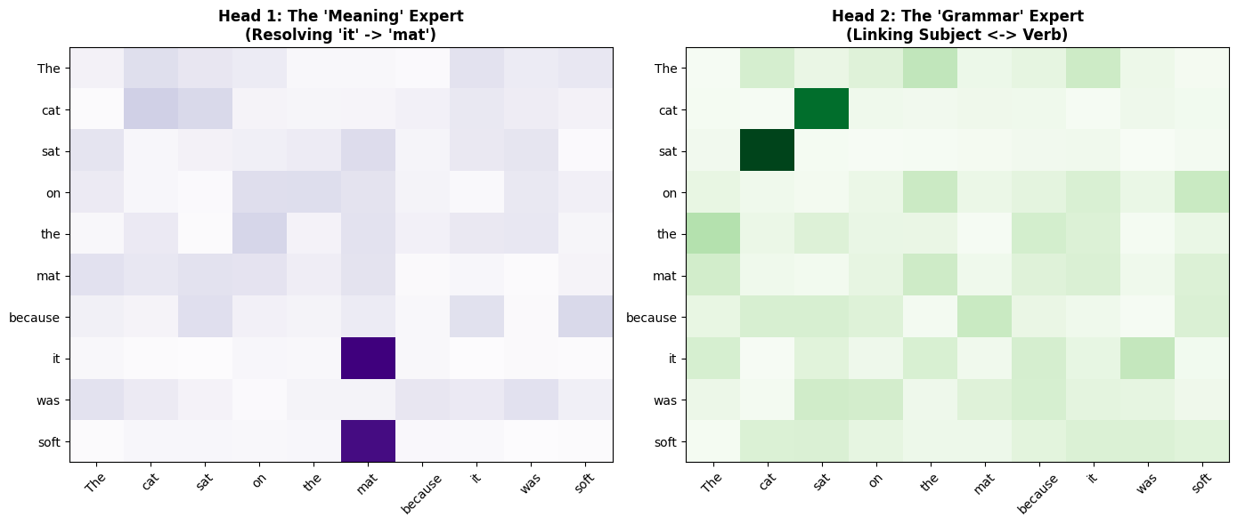
Part 3: Visualizing Multiple Perspectives¶

Let’s create a concrete example showing how two different heads learn different attention patterns on the same sentence.

Sentence: “The cat sat on the mat because it was soft.”

We’ll manually construct attention patterns to demonstrate what trained heads might learn:

Head 1 (Semantic): Focuses on meaning - connects “it” to “mat”
Head 2 (Syntactic): Focuses on grammar - connects “sat” to “cat” (subject-verb)

import numpy as np
import torch
import torch.nn.functional as F

tokens = ["The", "cat", "sat", "on", "the", "mat", "because", "it", "was", "soft"]
n_tokens = len(tokens)

print("Sentence:", " ".join(tokens))
print(f"Tokens: {n_tokens}")
print()

# Head 1: Semantic relationships (it -> mat, soft -> mat)
print("=" * 70)
print("HEAD 1: Semantic Expert")
print("=" * 70)
head1_logits = torch.zeros(n_tokens, n_tokens)
# "it" should attend to "mat" (physical reference)
head1_logits[tokens.index("it"), tokens.index("mat")] = 8.0
# "soft" should attend to "mat" (property)
head1_logits[tokens.index("soft"), tokens.index("mat")] = 6.0
# Everyone else attends mostly to themselves
for i in range(n_tokens):
    if tokens[i] not in ["it", "soft"]:
        head1_logits[i, i] = 5.0

head1_weights = F.softmax(head1_logits, dim=-1)

print("\nKey patterns in Head 1:")
for i, token in enumerate(tokens):
    max_attn_idx = torch.argmax(head1_weights[i]).item()
    max_attn_val = head1_weights[i, max_attn_idx].item()
    if max_attn_val > 0.5:
        print(f"  '{token}' → '{tokens[max_attn_idx]}' ({max_attn_val:.2f})")

# Head 2: Syntactic relationships (verb -> subject)
print("\n" + "=" * 70)
print("HEAD 2: Syntactic Expert")
print("=" * 70)
head2_logits = torch.zeros(n_tokens, n_tokens)
# "sat" should attend to "cat" (subject of verb)
head2_logits[tokens.index("sat"), tokens.index("cat")] = 8.0
# "cat" should attend to "sat" (verb of subject)
head2_logits[tokens.index("cat"), tokens.index("sat")] = 6.0
# Everyone else attends mostly to themselves
for i in range(n_tokens):
    if tokens[i] not in ["cat", "sat"]:
        head2_logits[i, i] = 5.0

head2_weights = F.softmax(head2_logits, dim=-1)

print("\nKey patterns in Head 2:")
for i, token in enumerate(tokens):
    max_attn_idx = torch.argmax(head2_weights[i]).item()
    max_attn_val = head2_weights[i, max_attn_idx].item()
    if max_attn_val > 0.5:
        print(f"  '{token}' → '{tokens[max_attn_idx]}' ({max_attn_val:.2f})")

print("\n" + "=" * 70)
print("✓ Different heads capture different linguistic relationships!")
print("=" * 70)

Sentence: The cat sat on the mat because it was soft
Tokens: 10

======================================================================
HEAD 1: Semantic Expert
======================================================================

Key patterns in Head 1:
  'The' → 'The' (0.94)
  'cat' → 'cat' (0.94)
  'sat' → 'sat' (0.94)
  'on' → 'on' (0.94)
  'the' → 'the' (0.94)
  'mat' → 'mat' (0.94)
  'because' → 'because' (0.94)
  'it' → 'mat' (1.00)
  'was' → 'was' (0.94)
  'soft' → 'mat' (0.98)

======================================================================
HEAD 2: Syntactic Expert
======================================================================

Key patterns in Head 2:
  'The' → 'The' (0.94)
  'cat' → 'sat' (0.98)
  'sat' → 'cat' (1.00)
  'on' → 'on' (0.94)
  'the' → 'the' (0.94)
  'mat' → 'mat' (0.94)
  'because' → 'because' (0.94)
  'it' → 'it' (0.94)
  'was' → 'was' (0.94)
  'soft' → 'soft' (0.94)

======================================================================
✓ Different heads capture different linguistic relationships!
======================================================================

Now let’s visualize these patterns side-by-side:

import matplotlib.pyplot as plt
import numpy as np

tokens = ["The", "cat", "sat", "on", "the", "mat", "because", "it", "was", "soft"]
fig, (ax1, ax2) = plt.subplots(1, 2, figsize=(14, 6))

# Head 1: Reference Resolution (it -> mat)
# Simulating a head that understands physical properties
head1 = np.zeros((len(tokens), len(tokens)))
head1[tokens.index("it"), tokens.index("mat")] = 0.95
head1[tokens.index("soft"), tokens.index("mat")] = 0.8
# Add some background noise
np.random.seed(42)
head1 += np.random.rand(len(tokens), len(tokens)) * 0.05
# Normalize
head1 = head1 / head1.sum(axis=1, keepdims=True)

# Head 2: Syntax / Subject-Verb (sat -> cat)
# Simulating a head that connects verbs to their subjects
head2 = np.zeros((len(tokens), len(tokens)))
head2[tokens.index("cat"), tokens.index("sat")] = 0.6
head2[tokens.index("sat"), tokens.index("cat")] = 0.9
head2 += np.random.rand(len(tokens), len(tokens)) * 0.05
head2 = head2 / head2.sum(axis=1, keepdims=True)

# Plotting Head 1
im1 = ax1.imshow(head1, cmap='Purples', aspect='auto')
ax1.set_title("Head 1: The 'Meaning' Expert\n(Resolving 'it' -> 'mat')", fontsize=12, fontweight='bold')
ax1.set_xticks(range(len(tokens)))
ax1.set_xticklabels(tokens, rotation=45)
ax1.set_yticks(range(len(tokens)))
ax1.set_yticklabels(tokens)
ax1.grid(False)

# Plotting Head 2
im2 = ax2.imshow(head2, cmap='Greens', aspect='auto')
ax2.set_title("Head 2: The 'Grammar' Expert\n(Linking Subject <-> Verb)", fontsize=12, fontweight='bold')
ax2.set_xticks(range(len(tokens)))
ax2.set_xticklabels(tokens, rotation=45)
ax2.set_yticks(range(len(tokens)))
ax2.set_yticklabels(tokens)
ax2.grid(False)

plt.tight_layout()
plt.show()

Part 4: Implementation in PyTorch¶

In L03, we implemented single-head attention on batches [B, S, D]:

B = Batch size (multiple sequences processed in parallel)
S = Sequence length (number of tokens)
D = Embedding dimension (features per token)

Multi-head attention adds one more dimension: H (number of heads).

Our tensors now become [B, H, S, d_k] where:

H = Number of heads (e.g., 8)
d_k = Dimensions per head (d_k = D / H = 64)

The key challenge: How do we efficiently compute H attention mechanisms in parallel?

The answer: Clever tensor reshaping with view() and transpose(). Instead of looping over heads, PyTorch reshapes tensors so all heads run in parallel.

We’ll use $H=8$ heads and $d_k = D/H = 64$ dims per head.

Project (Mix): $[B,S,D] \rightarrow [B,S,D]$
Apply $W^Q, W^K, W^V$ to produce $Q,K,V$ . Each projected feature can use all $D$ input dimensions.
Split: $[B,S,D] \rightarrow [B,S,H,d_k]$
view(B, S, H, d_k) splits the last dimension into heads × per-head dims.
Reorder: $[B,S,H,d_k] \rightarrow [B,H,S,d_k]$
transpose(1, 2) moves the heads dimension next to the batch dimension, so the tensor behaves like $B\times H$ independent attention problems.

# Show the exact tensor operations in PyTorch (tiny shapes)
B, S, D = 2, 10, 512
H = 8
d_k = D // H

x_big = torch.randn(B, S, D)

Wq = torch.randn(D, D)
q = x_big @ Wq                      # [B,S,D]
q_view = q.view(B, S, H, d_k)       # [B,S,H,d_k]
q_reordered = q_view.transpose(1, 2)  # [B,H,S,d_k]

print("x_big:", x_big.shape)
print("q:", q.shape)
print("q_view:", q_view.shape)
print("q_reordered:", q_reordered.shape)

# The per-head slice is now easy:
print("One head slice:", q_reordered[:, 0].shape, "(= [B,S,d_k])")

x_big: torch.Size([2, 10, 512])
q: torch.Size([2, 10, 512])
q_view: torch.Size([2, 10, 8, 64])
q_reordered: torch.Size([2, 8, 10, 64])
One head slice: torch.Size([2, 10, 64]) (= [B,S,d_k])

Now let’s visualize these tensor transformations:

from matplotlib import pyplot as plt
import numpy as np
from matplotlib import patches

import matplotlib.patheffects as pe

def plot_tensor_transformations(light_scale=2.3, figsize=(20.7, 10.35)):
    """
    Visualize the view() and transpose() operations as a clean 2D horizontal flow.

    Fixes:
      - Orange box main dimension label contrast (adds light bbox + darker text)
      - Green head labels larger + outlined for readability
      - light_scale=2.0 doubles grey/italic captions + top annotation boxes
    """
    fig, ax = plt.subplots(1, 1, figsize=figsize)
    ax.set_xlim(0, 17 * (figsize[0]/18))
    ax.set_ylim(0, 9 * (figsize[1]/9))
    ax.axis("off")

    # ---- layout ----
    y_center = 4.75 * (figsize[1]/9)
    box_width = 3.5 * (figsize[0]/18)
    box_height = 1.4 * (figsize[1]/9)

    # Fonts
    main_dim_fs = 18 # 16 * 1.15 = 18.4
    header_fs = 17 # 15 * 1.15 = 17.25
    op_fs = 14 # 12 * 1.15 = 13.8
    light_fs = int(round(10 * light_scale))  # grey/italic captions
    anno_fs = int(round(9 * light_scale))    # top annotation boxes
    key_fs = 15 # 13 * 1.15 = 14.95
    head_fs = 13 # 11 * 1.15 = 12.65

    def op_bbox(face, edge):
        return dict(facecolor=face, edgecolor=edge, boxstyle="round,pad=0.35", linewidth=2)

    # -------------------------
    # Step 1: [2, 10, 512]
    # -------------------------
    x1 = 1.0 * (figsize[0]/18)
    ax.add_patch(
        patches.Rectangle(
            (x1, y_center - box_height / 2),
            box_width,
            box_height,
            facecolor="#90CAF9",
            edgecolor="#1976D2",
            linewidth=3,
        )
    )

    ax.text(
        x1 + box_width / 2,
        y_center,
        "[2, 10, 512]",
        ha="center",
        va="center",
        fontsize=main_dim_fs,
        fontweight="bold",
        color="#0D47A1",
    )

    ax.text(
        x1 + box_width / 2,
        y_center + box_height / 2 + 0.70 * (figsize[1]/9),
        r"After $W^Q(x)$",
        ha="center",
        va="bottom",
        fontsize=header_fs,
        fontweight="bold",
    )

    ax.text(
        x1 + box_width / 2,
        y_center - box_height / 2 - 0.45 * (figsize[1]/9),
        "Flat 512 dims",
        ha="center",
        va="top",
        fontsize=light_fs,
        style="italic",
        color="#555",
    )

    # -------------------------
    # Arrow + .view()
    # -------------------------
    arrow1_start = x1 + box_width + 0.15 * (figsize[0]/18)
    arrow1_end = x1 + box_width + 0.95 * (figsize[0]/18)
    ax.add_patch(
        patches.FancyArrowPatch(
            (arrow1_start, y_center),
            (arrow1_end, y_center),
            arrowstyle="->,head_width=0.55,head_length=0.65",
            lw=4,
            color="#FF6F00",
        )
    )

    ax.text(
        (arrow1_start + arrow1_end) / 2,
        y_center + 0.85 * (figsize[1]/9),
        ".view(2, 10, 8, 64)",
        ha="center",
        va="bottom",
        fontsize=op_fs,
        fontweight="bold",
        color="#FF6F00",
        bbox=op_bbox("#FFF3E0", "#FF6F00"),
    )

    # -------------------------
    # Step 2: [2, 10, 8, 64]
    # -------------------------
    x2 = arrow1_end + 0.15 * (figsize[0]/18)

    n_layers = 8
    layer_height = box_height / n_layers
    for i in range(n_layers):
        ax.add_patch(
            patches.Rectangle(
                (x2, y_center - box_height / 2 + i * layer_height),
                box_width,
                layer_height,
                facecolor="#FFB74D",
                edgecolor="#F57C00",
                linewidth=1.4,
                alpha=0.88,
            )
        )

    # Contrast fix: darker text + light background behind it
    ax.text(
        x2 + box_width / 2,
        y_center,
        "[2, 10, 8, 64]",
        ha="center",
        va="center",
        fontsize=main_dim_fs,
        fontweight="bold",
        color="#2D1B00",
        bbox=dict(facecolor="white", alpha=0.65, edgecolor="none", boxstyle="round,pad=0.22"),
    )

    ax.text(
        x2 + box_width / 2,
        y_center + box_height / 2 + 0.70 * (figsize[1]/9),
        "After .view()",
        ha="center",
        va="bottom",
        fontsize=header_fs,
        fontweight="bold",
    )

    ax.text(
        x2 + box_width / 2,
        y_center - box_height / 2 - 0.45 * (figsize[1]/9),
        "8 heads × 64 dims",
        ha="center",
        va="top",
        fontsize=light_fs,
        style="italic",
        color="#555",
    )

    # -------------------------
    # Arrow + .transpose()
    # -------------------------
    arrow2_start = x2 + box_width + 0.15 * (figsize[0]/18)
    arrow2_end = x2 + box_width + 1.05 * (figsize[0]/18)
    ax.add_patch(
        patches.FancyArrowPatch(
            (arrow2_start, y_center),
            (arrow2_end, y_center),
            arrowstyle="->,head_width=0.55,head_length=0.65",
            lw=4,
            color="#2E7D32",
        )
    )

    ax.text(
        (arrow2_start + arrow2_end) / 2,
        y_center + 0.85 * (figsize[1]/9),
        ".transpose(1, 2)",
        ha="center",
        va="bottom",
        fontsize=op_fs,
        fontweight="bold",
        color="#2E7D32",
        bbox=op_bbox("#E8F5E9", "#2E7D32"),
    )

    # -------------------------
    # Step 3: [2, 8, 10, 64]
    # -------------------------
    x3 = arrow2_end + 0.15 * (figsize[0]/18)

    n_segments = 8
    segment_width = box_width / n_segments
    for i in range(n_segments):
        ax.add_patch(
            patches.Rectangle(
                (x3 + i * segment_width, y_center - box_height / 2),
                segment_width,
                box_height,
                facecolor="#81C784",
                edgecolor="#388E3C",
                linewidth=1.8,
                alpha=0.92,
            )
        )
        t = ax.text(
            x3 + i * segment_width + segment_width / 2,
            y_center,
            f"H{i+1}",
            ha="center",
            va="center",
            fontsize=head_fs,
            fontweight="bold",
            color="white",
        )
        # Outline makes white text readable against mid-tone greens
        t.set_path_effects([pe.withStroke(linewidth=2.5, foreground="black")])

    ax.text(
        x3 + box_width / 2,
        y_center + box_height / 2 + 0.70 * (figsize[1]/9),
        "After .transpose(1, 2)",
        ha="center",
        va="bottom",
        fontsize=header_fs,
        fontweight="bold",
    )

    ax.text(
        x3 + box_width / 2,
        y_center + box_height / 2 + 1.10 * (figsize[1]/9),
        "[2, 8, 10, 64]",
        ha="center",
        va="bottom",
        fontsize=main_dim_fs,
        fontweight="bold",
        color="#1B5E20",
    )

    ax.text(
        x3 + box_width / 2,
        y_center - box_height / 2 - 0.45 * (figsize[1]/9),
        "Heads are independent!",
        ha="center",
        va="top",
        fontsize=light_fs,
        style="italic",
        color="#555",
    )

    # -------------------------
    # Top annotations
    # -------------------------
    top_y = y_center + box_height / 2 + 2.10 * (figsize[1]/9)
    ax.text(
        x1 + box_width / 2,
        top_y,
        "Batch=2, Seq=10\nD_model=512",
        ha="center",
        va="bottom",
        fontsize=anno_fs,
        color="#666",
        bbox=dict(facecolor="white", edgecolor="#90CAF9", boxstyle="round,pad=0.30", linewidth=1.2),
    )

    ax.text(
        x2 + box_width / 2,
        top_y,
        "Batch=2, Seq=10\nHeads=8, D_k=64",
        ha="center",
        va="bottom",
        fontsize=anno_fs,
        color="#666",
        bbox=dict(facecolor="white", edgecolor="#FFB74D", boxstyle="round,pad=0.30", linewidth=1.2),
    )

    ax.text(
        x3 + box_width / 2,
        top_y,
        "Batch=2, Heads=8\nSeq=10, D_k=64",
        ha="center",
        va="bottom",
        fontsize=anno_fs,
        color="#666",
        bbox=dict(facecolor="white", edgecolor="#81C784", boxstyle="round,pad=0.30", linewidth=1.2),
    )

    # -------------------------
    # Bottom key insight
    # -------------------------
    ax.text(
        8.5 * (figsize[0]/18),
        1.05 * (figsize[1]/9),
        "Key Insight: After transpose, PyTorch processes all 8 heads in parallel\n"
        "by treating [Batch × Heads] as a combined batch dimension.",
        ha="center",
        va="center",
        fontsize=key_fs,
        fontweight="bold",
        bbox=dict(facecolor="#E3F2FD", edgecolor="#1976D2", boxstyle="round,pad=0.70", linewidth=2),
    )

    plt.tight_layout()
    plt.show()

plot_tensor_transformations(light_scale=2.3, figsize=(20.7, 10.35))

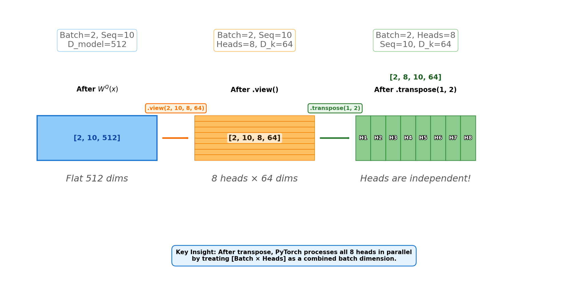
Shape Transformation Table¶

Let’s trace the exact tensor shapes through a concrete example with batch=2, seq=10, d_model=512, heads=8:

Operation	Shape	Description
Input `x`	`[2, 10, 512]`	Raw input: 2 sequences, each with 10 tokens, 512-dim embeddings
After `W_q(x)`	`[2, 10, 512]`	Linear projection (still flat)
After `.view(2, 10, 8, 64)`	`[2, 10, 8, 64]`	Reshape: Split 512 dims into 8 heads × 64 dims each
After `.transpose(1, 2)`	`[2, 8, 10, 64]`	Swap seq and heads: Now we have 8 “parallel attention mechanisms”
Attention computation	`[2, 8, 10, 64]`	Each head computes attention independently
After `.transpose(1, 2)`	`[2, 10, 8, 64]`	Swap back: Prepare for concatenation
After `.contiguous().view(2, 10, 512)`	`[2, 10, 512]`	Flatten: Merge 8 heads back into single 512-dim vector
After `W_o(x)`	`[2, 10, 512]`	Final projection

The key insight: dimensions 1 and 2 get swapped twice—once to parallelize the heads, and once to merge them back together.

# Why contiguous() matters (a runnable demo)
x_demo = torch.randn(2, 3, 4)
x_t = x_demo.transpose(1, 2)  # changes strides, doesn't move data
print("x_t.is_contiguous():", x_t.is_contiguous())

try:
    _ = x_t.view(2, 12)  # may error if not contiguous
    print("view() worked (unexpected in some layouts)")
except RuntimeError as e:
    print("view() failed as expected:", e)

x_c = x_t.contiguous()
print("x_c.is_contiguous():", x_c.is_contiguous())
print("x_c.view(2, 12).shape:", x_c.view(2, 12).shape)

x_t.is_contiguous(): False
view() failed as expected: view size is not compatible with input tensor's size and stride (at least one dimension spans across two contiguous subspaces). Use .reshape(...) instead.
x_c.is_contiguous(): True
x_c.view(2, 12).shape: torch.Size([2, 12])

import math
import torch
import torch.nn as nn
import torch.nn.functional as F

class MultiHeadAttention(nn.Module):
    def __init__(self, d_model, num_heads):
        super().__init__()
        assert d_model % num_heads == 0, "d_model must be divisible by num_heads"
        
        self.d_model = d_model
        self.num_heads = num_heads
        self.d_k = d_model // num_heads
        
        # We define 4 linear layers: Q, K, V projections and the final Output
        self.W_q = nn.Linear(d_model, d_model)
        self.W_k = nn.Linear(d_model, d_model)
        self.W_v = nn.Linear(d_model, d_model)
        self.W_o = nn.Linear(d_model, d_model)
        
    def forward(self, q, k, v, mask=None):
        batch_size = q.size(0)
        
        # 1. Project and Split
        # We transform [Batch, Seq, Model] -> [Batch, Seq, Heads, d_k]
        # Then we transpose to [Batch, Heads, Seq, d_k] for matrix multiplication
        Q = self.W_q(q).view(batch_size, -1, self.num_heads, self.d_k).transpose(1, 2)
        K = self.W_k(k).view(batch_size, -1, self.num_heads, self.d_k).transpose(1, 2)
        V = self.W_v(v).view(batch_size, -1, self.num_heads, self.d_k).transpose(1, 2)
        
        # 2. Scaled Dot-Product Attention (re-using logic from L03)
        # Scores shape: [Batch, Heads, Seq, Seq]
        scores = torch.matmul(Q, K.transpose(-2, -1)) / math.sqrt(self.d_k)
        
        if mask is not None:
            scores = scores.masked_fill(mask == 0, -1e9)
        
        attn_weights = torch.softmax(scores, dim=-1)
        
        # Apply weights to Values
        # Shape: [Batch, Heads, Seq, d_k]
        attn_output = torch.matmul(attn_weights, V)
        
        # 3. Concatenate
        # Transpose back: [Batch, Seq, Heads, d_k]
        # Flatten: [Batch, Seq, d_model]
        attn_output = attn_output.transpose(1, 2)
        attn_output = attn_output.contiguous()
        attn_output = attn_output.view(batch_size, -1, self.d_model)
        
        # 4. Final Projection (The "Mix")
        return self.W_o(attn_output)

# Demo: Test the MultiHeadAttention module
print("=" * 70)
print("TESTING MULTI-HEAD ATTENTION MODULE")
print("=" * 70)

torch.manual_seed(0)
d_model = 32
num_heads = 4
batch_size = 2
seq_len = 5

mha = MultiHeadAttention(d_model=d_model, num_heads=num_heads)
x_in = torch.randn(batch_size, seq_len, d_model)

print(f"\nConfiguration:")
print(f"  d_model: {d_model}")
print(f"  num_heads: {num_heads}")
print(f"  d_k per head: {d_model // num_heads}")
print(f"\nInput shape: {x_in.shape} = [Batch, Seq, D_model]")

# Forward pass (self-attention: q=k=v=x)
y_out = mha(x_in, x_in, x_in)

print(f"Output shape: {y_out.shape} = [Batch, Seq, D_model]")
print(f"\n✓ Shape preserved: {x_in.shape} → {y_out.shape}")

# Show that output is different from input (attention mixed information)
diff = (y_out - x_in).abs().mean().item()
print(f"✓ Output differs from input (mean abs diff: {diff:.4f})")
print("  This means attention successfully mixed contextual information!")

# Show parameter count
total_params = sum(p.numel() for p in mha.parameters())
print(f"\n✓ Total parameters: {total_params:,}")
print(f"  Breakdown:")
print(f"    W_q: {d_model} × {d_model} = {d_model*d_model:,}")
print(f"    W_k: {d_model} × {d_model} = {d_model*d_model:,}")
print(f"    W_v: {d_model} × {d_model} = {d_model*d_model:,}")
print(f"    W_o: {d_model} × {d_model} = {d_model*d_model:,}")
print(f"    Total: {4*d_model*d_model:,}")

print("\n" + "=" * 70)

======================================================================
TESTING MULTI-HEAD ATTENTION MODULE
======================================================================

Configuration:
  d_model: 32
  num_heads: 4
  d_k per head: 8

Input shape: torch.Size([2, 5, 32]) = [Batch, Seq, D_model]
Output shape: torch.Size([2, 5, 32]) = [Batch, Seq, D_model]

✓ Shape preserved: torch.Size([2, 5, 32]) → torch.Size([2, 5, 32])
✓ Output differs from input (mean abs diff: 0.7951)
  This means attention successfully mixed contextual information!

✓ Total parameters: 4,224
  Breakdown:
    W_q: 32 × 32 = 1,024
    W_k: 32 × 32 = 1,024
    W_v: 32 × 32 = 1,024
    W_o: 32 × 32 = 1,024
    Total: 4,096

======================================================================

# Verification: Loop-based vs Vectorized implementation produce identical results
def mha_forward_loop(mha_module, x, mask=None):
    """
    A loop-based implementation that's easier to understand.
    This should produce IDENTICAL results to the vectorized version.
    """
    B, S, D = x.shape
    H = mha_module.num_heads
    d_k = mha_module.d_k

    # Same projections as the module
    Q = mha_module.W_q(x)  # [B,S,D]
    K = mha_module.W_k(x)
    V = mha_module.W_v(x)

    # Split into heads (without transpose yet, to make slicing intuitive)
    Qs = Q.view(B, S, H, d_k)
    Ks = K.view(B, S, H, d_k)
    Vs = V.view(B, S, H, d_k)

    heads = []
    for h in range(H):
        qh = Qs[:, :, h, :]  # [B,S,d_k]
        kh = Ks[:, :, h, :]
        vh = Vs[:, :, h, :]

        scores = qh @ kh.transpose(-2, -1) / math.sqrt(d_k)  # [B,S,S]
        if mask is not None:
            scores = scores.masked_fill(mask == 0, -1e9)
        attn = torch.softmax(scores, dim=-1)
        out = attn @ vh  # [B,S,d_k]
        heads.append(out)

    concat = torch.cat(heads, dim=-1)  # [B,S,D]
    return mha_module.W_o(concat)

print("=" * 70)
print("VERIFICATION: Vectorized vs Loop-Based Implementation")
print("=" * 70)

torch.manual_seed(123)
mha = MultiHeadAttention(d_model=32, num_heads=4)
x_in = torch.randn(2, 6, 32)

print(f"\nInput: {x_in.shape}")

y_vec = mha(x_in, x_in, x_in)
y_loop = mha_forward_loop(mha, x_in)

print(f"Vectorized output: {y_vec.shape}")
print(f"Loop-based output: {y_loop.shape}")

max_diff = (y_vec - y_loop).abs().max().item()
mean_diff = (y_vec - y_loop).abs().mean().item()

print(f"\nDifference between implementations:")
print(f"  Max absolute diff: {max_diff:.10f}")
print(f"  Mean absolute diff: {mean_diff:.10f}")
print(f"  Results match: {torch.allclose(y_vec, y_loop, atol=1e-6)}")

print("\n✓ Both implementations produce identical results!")
print("  The vectorized version is just faster on GPUs")
print("=" * 70)

======================================================================
VERIFICATION: Vectorized vs Loop-Based Implementation
======================================================================

Input: torch.Size([2, 6, 32])
Vectorized output: torch.Size([2, 6, 32])
Loop-based output: torch.Size([2, 6, 32])

Difference between implementations:
  Max absolute diff: 0.0000000000
  Mean absolute diff: 0.0000000000
  Results match: True

✓ Both implementations produce identical results!
  The vectorized version is just faster on GPUs
======================================================================

# Demo: Causal masking (for GPT-style models)
print("=" * 70)
print("CAUSAL MASKING EXAMPLE")
print("=" * 70)

B, S, D = 2, 6, 32
mha = MultiHeadAttention(d_model=D, num_heads=4)
x_in = torch.randn(B, S, D)

# causal mask: [S,S] lower triangular -> broadcastable to [B,1,S,S]
causal = torch.tril(torch.ones(S, S)).unsqueeze(0).unsqueeze(1)

print(f"\nCausal mask shape: {causal.shape} (will broadcast to [B, H, S, S])")
print(f"Causal mask (first 4x4 for visualization):")
print(causal[0, 0, :4, :4].int())
print("  1 = can attend, 0 = cannot attend (future tokens masked)")

y_masked = mha(x_in, x_in, x_in, mask=causal)
y_unmasked = mha(x_in, x_in, x_in, mask=None)

print(f"\nMasked output: {y_masked.shape}")
print(f"Unmasked output: {y_unmasked.shape}")

diff = (y_masked - y_unmasked).abs().mean().item()
print(f"\nMean absolute difference: {diff:.4f}")
print("✓ Masking changes the output - tokens can't peek at the future!")
print("\nNote: Causal masking is used in GPT models to prevent")
print("      tokens from attending to future positions during training.")
print("=" * 70)

======================================================================
CAUSAL MASKING EXAMPLE
======================================================================


Causal mask shape: torch.Size([1, 1, 6, 6]) (will broadcast to [B, H, S, S])
Causal mask (first 4x4 for visualization):
tensor([[1, 0, 0, 0],
        [1, 1, 0, 0],
        [1, 1, 1, 0],
        [1, 1, 1, 1]], dtype=torch.int32)
  1 = can attend, 0 = cannot attend (future tokens masked)

Masked output: torch.Size([2, 6, 32])
Unmasked output: torch.Size([2, 6, 32])

Mean absolute difference: 0.0999
✓ Masking changes the output - tokens can't peek at the future!

Note: Causal masking is used in GPT models to prevent
      tokens from attending to future positions during training.
======================================================================

Why .contiguous()? Understanding Memory Layout

When we transpose a tensor in PyTorch, we aren’t actually moving data in memory; we are just changing the “stride” (how the computer steps through memory).

Memory Layout Explanation:

Tensors are stored as 1D arrays in memory. Multi-dimensional tensors use “strides” to map from indices to memory locations.
When you call .transpose(), PyTorch creates a new view with different strides, but the underlying data stays in the same physical order in memory.
The view() operation requires the data to be laid out in a specific order in memory (row-major, also called C-contiguous).
If the tensor isn’t contiguous after transpose, calling .view() would give incorrect results or raise an error.

What .contiguous() does:

Creates a new tensor with data physically rearranged in memory to match the current logical shape.
This is a copy operation, so it has a performance cost, but it’s necessary to ensure correctness.

Example:

x = torch.randn(2, 3, 4)
x_t = x.transpose(1, 2)  # Creates a view, not contiguous
print(x_t.is_contiguous())  # False
x_c = x_t.contiguous()      # Creates a contiguous copy
print(x_c.is_contiguous())  # True

This is a PyTorch implementation detail; the math doesn’t care about memory layout, but the computer does!

Summary¶

Multiple Heads: We split our embedding into $h$ smaller chunks to allow the model to focus on different linguistic features simultaneously.
Projection: We use learned linear layers ( $W^Q, W^K, W^V, W^O$ ) to project the input into these specialized subspaces.
Parallelism: We use tensor reshaping (view and transpose) to compute attention for all heads at once, rather than looping through them.

Next Up: L05 – Layer Norm & Residuals. We have built the engine (Attention), but if we stack 100 of these layers on top of each other, the gradients will vanish or explode. In L05, we will add the “plumbing” (Normalization and Skip Connections) that allows Deep Learning to actually get deep.