L05 - Normalization & Residuals: The Plumbing of Deep Networks

How to stop gradients from vanishing and signals from exploding

In L04, we built the Multi-Head Attention engine. But there’s a problem: in a deep LLM, we stack these attention layers dozens of times. As the data flows through these transformations, the numbers can drift—they might become tiny (vanishing gradients) or massive (exploding activations).

If the numbers get weird, the model stops learning. To fix this, Transformers use a critical pattern called “Add & Norm”—a combination of two techniques that work together:

1. Residual (Skip) Connections (“Add”): Provide a direct path for gradients to flow backward

2. Layer Normalization (“Norm”): Keep activations in a healthy range

Think of it like this: Multi-Head Attention does the thinking, while Add & Norm does the housekeeping to keep the network trainable.

By the end of this post, you’ll understand:

• The intuition behind Add & Norm as a unit

• Why Residual Connections allow for incredibly deep models (100+ layers)

• How to implement LayerNorm from scratch

• How to wrap L04’s MultiHeadAttention in a complete Transformer block

import os
import logging
import warnings

logging.getLogger("matplotlib.font_manager").setLevel(logging.ERROR)

import torch
import torch.nn as nn
import matplotlib
import numpy as np
import matplotlib.pyplot as plt

plt.rcParams['figure.facecolor'] = 'white'
plt.rcParams['axes.facecolor'] = 'white'

Part 1: Residual Connections (The Skip)¶

In a standard network, data flows like this:

In a Transformer, we do this:

We literally add the input back to the output.

Why?

Imagine you are trying to describe a complex concept. If you only give the “transformed” explanation, you might lose the original context. By adding the input back, we provide a “highway” for the original signal to travel through.

Visualizing Gradient Flow: With vs. Without Residuals¶

Let’s see the dramatic difference residual connections make in a deep network:

import numpy as np
import matplotlib.pyplot as plt

# Simulate gradient magnitudes through layers
num_layers = 20
layers = np.arange(1, num_layers + 1)

# Without residuals: exponential decay (vanishing gradients)
# Each layer multiplies gradient by ~0.8 (typical for deep networks)
gradient_without_residual = np.power(0.8, layers - 1)

# With residuals: gradient stays stable due to identity path
# The "+1" term in the derivative prevents vanishing
gradient_with_residual = 0.7 + 0.3 * np.power(0.9, layers - 1)

fig, (ax1, ax2) = plt.subplots(1, 2, figsize=(14, 5))

# Plot 1: Gradient Magnitude
ax1.plot(layers, gradient_without_residual, 'o-', label='Without Residuals',
         color='red', linewidth=2, markersize=6)
ax1.plot(layers, gradient_with_residual, 's-', label='With Residuals',
         color='green', linewidth=2, markersize=6)
ax1.axhline(y=0.1, color='gray', linestyle='--', alpha=0.5, label='Vanishing Threshold')
ax1.set_xlabel('Layer Depth', fontsize=12)
ax1.set_ylabel('Gradient Magnitude', fontsize=12)
ax1.set_title('Gradient Flow Through Deep Network', fontsize=14, fontweight='bold')
ax1.legend()
ax1.grid(True, alpha=0.3)
ax1.set_yscale('log')

# Plot 2: Layer-by-layer comparison
bar_width = 0.35
x_pos = np.arange(len(layers[:10]))
ax2.bar(x_pos - bar_width/2, gradient_without_residual[:10], bar_width,
        label='Without Residuals', color='red', alpha=0.7)
ax2.bar(x_pos + bar_width/2, gradient_with_residual[:10], bar_width,
        label='With Residuals', color='green', alpha=0.7)
ax2.set_xlabel('Layer Number', fontsize=12)
ax2.set_ylabel('Gradient Magnitude', fontsize=12)
ax2.set_title('First 10 Layers (Zoomed)', fontsize=14, fontweight='bold')
ax2.set_xticks(x_pos)
ax2.set_xticklabels(layers[:10])
ax2.legend()
ax2.grid(True, alpha=0.3, axis='y')

plt.tight_layout()
plt.show()

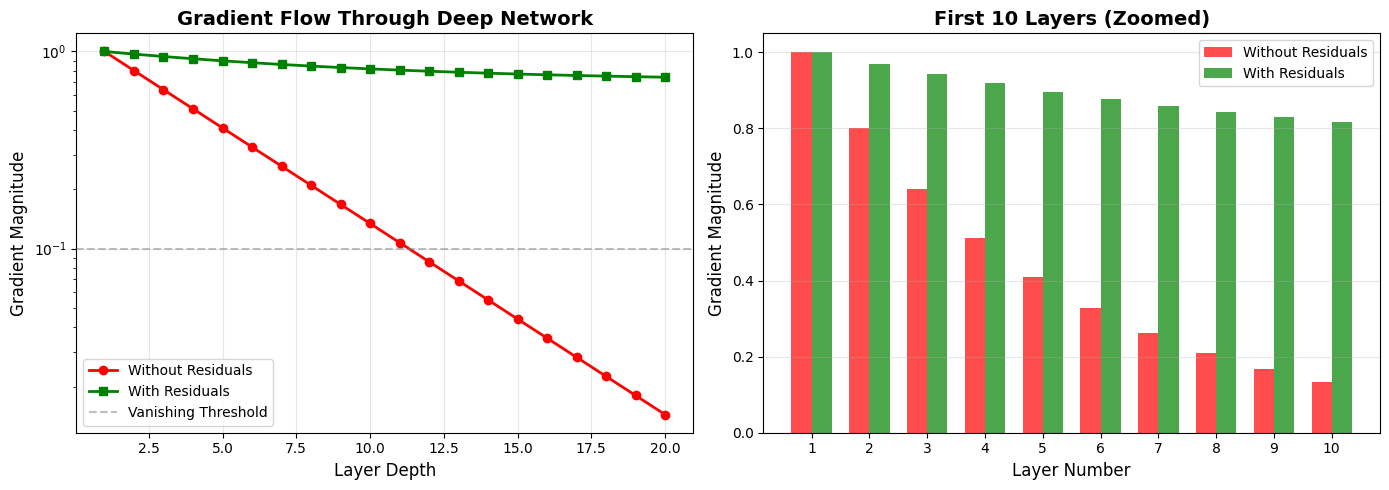
Key observations:

• Without residuals (red): Gradients decay exponentially, reaching near-zero by layer 10-15

• With residuals (green): Gradients remain strong even in deep layers

• This is why we can train 100+ layer transformers successfully!

Part 2: Layer Normalization (The Leveler)¶

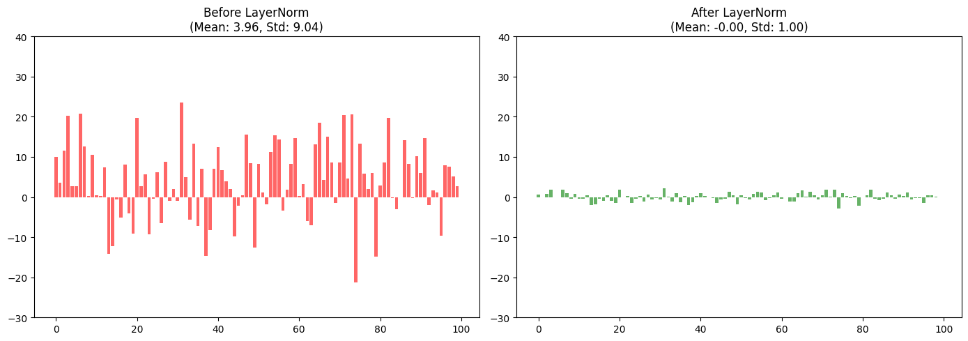
LayerNorm ensures that for every token, the mean of its features is 0 and the standard deviation is 1. This prevents any single feature or layer from dominating the calculation.

Unlike BatchNorm (common in CNNs), LayerNorm calculates statistics across the features of a single token. This makes it perfect for sequences of varying lengths.

LayerNorm vs. BatchNorm: What’s the Difference?¶

Both normalization techniques aim to stabilize training, but they compute statistics over different dimensions:

Why LayerNorm for Transformers?

• Variable sequence lengths: Different sentences have different lengths. BatchNorm would struggle with varying dimensions.

• Batch independence: Each example can be normalized independently, making it work even with tiny batches (e.g., batch_size=1 during inference).

• Recurrent/sequential nature: In sequences, we care about the distribution of features within each token, not across different tokens in a batch.

Visual Comparison:

BatchNorm (shape [4, 512]):          LayerNorm (shape [4, 512]):
┌─────────────────┐                  ┌─────────────────┐
│ Example 1       │                  │ Example 1       │ ← Normalize these 512 values
│ Example 2       │ ↑                │ Example 2       │ ← Normalize these 512 values
│ Example 3       │ │ Normalize      │ Example 3       │ ← Normalize these 512 values
│ Example 4       │ │ each column    │ Example 4       │ ← Normalize these 512 values
└─────────────────┘ ↓                └─────────────────┘

The Formula

For a vector $x$ (the features of a single token):

Where:

• $\mu$ = mean of the features: $\mu = \frac{1}{d}\sum_{i=1}^{d} x_i$

• $\sigma^2$ = variance of the features: $\sigma^2 = \frac{1}{d}\sum_{i=1}^{d} (x_i - \mu)^2$

• $\epsilon$ = small constant (e.g., 10^-6) to prevent division by zero

• $\gamma$ = learnable scale parameter (initialized to 1)

• $\beta$ = learnable shift parameter (initialized to 0)

Steps:

1. Calculate mean $\mu$ and variance $\sigma^2$ across all features

2. Normalize: subtract mean and divide by standard deviation

3. Scale and shift: $\gamma$ and $\beta$ let the model adjust the range if needed for learning

Part 3: Visualizing the “Add & Norm”¶

First, let’s see the complete Add & Norm pipeline in action:

# Simulate the complete Add & Norm pipeline
np.random.seed(42)
n_features = 64

# Step 1: Original input (from previous layer)
x_input = np.random.normal(loc=0, scale=1, size=n_features)

# Step 2: After transformation (e.g., attention output)
# This might have different statistics
transformed = np.random.normal(loc=2, scale=5, size=n_features)

# Step 3: ADD residual connection
x_after_add = x_input + transformed

# Step 4: NORM - Layer Normalization
mean = x_after_add.mean()
std = x_after_add.std()
x_after_norm = (x_after_add - mean) / std

# Create visualization
fig, axes = plt.subplots(2, 2, figsize=(14, 10))

# Plot 1: Input
axes[0, 0].bar(range(n_features), x_input, color='#3498db', alpha=0.7)
axes[0, 0].set_title(f"Step 1: Input\nMean: {x_input.mean():.2f}, Std: {x_input.std():.2f}",
                      fontsize=12, fontweight='bold')
axes[0, 0].set_ylim(-15, 20)
axes[0, 0].grid(True, alpha=0.3, axis='y')
axes[0, 0].set_ylabel('Value', fontsize=11)

# Plot 2: After Transformation
axes[0, 1].bar(range(n_features), transformed, color='#9b59b6', alpha=0.7)
axes[0, 1].set_title(f"Step 2: After Transformation (e.g., Attention)\nMean: {transformed.mean():.2f}, Std: {transformed.std():.2f}",
                      fontsize=12, fontweight='bold')
axes[0, 1].set_ylim(-15, 20)
axes[0, 1].grid(True, alpha=0.3, axis='y')
axes[0, 1].set_ylabel('Value', fontsize=11)

# Plot 3: After ADD (residual)
axes[1, 0].bar(range(n_features), x_after_add, color='#e74c3c', alpha=0.7)
axes[1, 0].set_title(f"Step 3: After ADD (x + F(x))\nMean: {x_after_add.mean():.2f}, Std: {x_after_add.std():.2f}",
                      fontsize=12, fontweight='bold')
axes[1, 0].set_ylim(-15, 20)
axes[1, 0].grid(True, alpha=0.3, axis='y')
axes[1, 0].set_xlabel('Feature Index', fontsize=11)
axes[1, 0].set_ylabel('Value', fontsize=11)

# Plot 4: After NORM
axes[1, 1].bar(range(n_features), x_after_norm, color='#27ae60', alpha=0.7)
axes[1, 1].set_title(f"Step 4: After NORM (LayerNorm)\nMean: {x_after_norm.mean():.2f}, Std: {x_after_norm.std():.2f}",
                      fontsize=12, fontweight='bold')
axes[1, 1].set_ylim(-15, 20)
axes[1, 1].grid(True, alpha=0.3, axis='y')
axes[1, 1].set_xlabel('Feature Index', fontsize=11)
axes[1, 1].set_ylabel('Value', fontsize=11)

# Add annotations
axes[1, 0].annotate('Residual brings back\noriginal signal',
                     xy=(32, x_after_add.max()-2), fontsize=10,
                     bbox=dict(boxstyle='round', facecolor='wheat', alpha=0.8))
axes[1, 1].annotate('Normalized to\nmean=0, std=1',
                     xy=(32, 2), fontsize=10,
                     bbox=dict(boxstyle='round', facecolor='lightgreen', alpha=0.8))

plt.tight_layout()
plt.show()

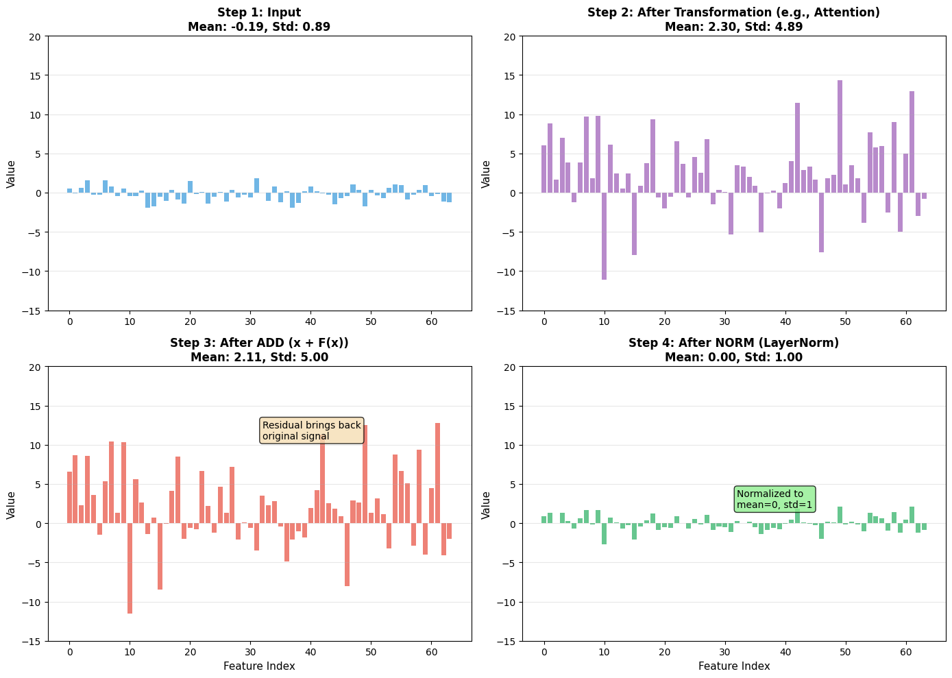
Key Observations:

• Step 3 (ADD): The residual connection preserves the original signal, even if the transformation changed the statistics

• Step 4 (NORM): LayerNorm brings everything back to a standard range (mean≈0, std≈1), preventing runaway values in deep networks

• Together: ADD ensures gradient flow, NORM ensures numerical stability

Now let’s zoom in on LayerNorm specifically:

# Create a "wild" vector of 100 features
np.random.seed(42)
wild_vector = np.random.normal(loc=5, scale=10, size=100)

# Normalize manually
mean = wild_vector.mean()
std = wild_vector.std()
norm_vector = (wild_vector - mean) / std

fig, (ax1, ax2) = plt.subplots(1, 2, figsize=(14, 5))

ax1.bar(range(100), wild_vector, color='red', alpha=0.6)
ax1.set_title(f"Before LayerNorm\n(Mean: {mean:.2f}, Std: {std:.2f})")
ax1.set_ylim(-30, 40)

ax2.bar(range(100), norm_vector, color='green', alpha=0.6)
ax2.set_title(f"After LayerNorm\n(Mean: {norm_vector.mean():.2f}, Std: {norm_vector.std():.2f})")
ax2.set_ylim(-30, 40)

plt.tight_layout()
plt.show()

Part 4: Building LayerNorm from Scratch¶

While PyTorch has nn.LayerNorm, building it yourself helps you understand exactly where those learnable parameters () live.

class LayerNorm(nn.Module):
    def __init__(self, d_model, eps=1e-6):
        super().__init__()
        self.gamma = nn.Parameter(torch.ones(d_model))
        self.beta = nn.Parameter(torch.zeros(d_model))
        self.eps = eps

    def forward(self, x):
        # x shape: [batch, seq_len, d_model]
        mean = x.mean(-1, keepdim=True)
        std = x.std(-1, keepdim=True)
        
        # Normalize
        x_norm = (x - mean) / (std + self.eps)
        
        # Scale and Shift
        return self.gamma * x_norm + self.beta

Let’s test it:

# Test LayerNorm implementation
class LayerNorm(nn.Module):
    def __init__(self, d_model, eps=1e-6):
        super().__init__()
        self.gamma = nn.Parameter(torch.ones(d_model))
        self.beta = nn.Parameter(torch.zeros(d_model))
        self.eps = eps

    def forward(self, x):
        # x shape: [batch, seq_len, d_model]
        mean = x.mean(-1, keepdim=True)
        std = x.std(-1, keepdim=True)

        # Normalize
        x_norm = (x - mean) / (std + self.eps)

        # Scale and Shift
        return self.gamma * x_norm + self.beta

# Create test data
torch.manual_seed(0)
batch, seq_len, d_model = 2, 4, 8
x_test = torch.randn(batch, seq_len, d_model) * 10 + 5  # Wild distribution

# Apply LayerNorm
ln = LayerNorm(d_model)
x_normed = ln(x_test)

print("Before LayerNorm:")
print(f"  Mean: {x_test.mean(-1)[0, 0]:.3f}")
print(f"  Std:  {x_test.std(-1)[0, 0]:.3f}")
print()
print("After LayerNorm:")
print(f"  Mean: {x_normed.mean(-1)[0, 0]:.3f}")
print(f"  Std:  {x_normed.std(-1)[0, 0]:.3f}")
print()
print("✓ LayerNorm normalized to mean≈0, std≈1")

Before LayerNorm:
  Mean: 0.184
  Std:  9.830

After LayerNorm:
  Mean: -0.000
  Std:  1.000

✓ LayerNorm normalized to mean≈0, std≈1

Part 4b: Putting It Together - The Complete Transformer Block¶

Now let’s combine Add & Norm with the MultiHeadAttention from L04 to build a complete Transformer block:

# Import MultiHeadAttention from L04 (we'll reimplement it here for completeness)
class MultiHeadAttention(nn.Module):
    def __init__(self, d_model, num_heads):
        super().__init__()
        assert d_model % num_heads == 0

        self.d_model = d_model
        self.num_heads = num_heads
        self.d_k = d_model // num_heads

        self.W_q = nn.Linear(d_model, d_model)
        self.W_k = nn.Linear(d_model, d_model)
        self.W_v = nn.Linear(d_model, d_model)
        self.W_o = nn.Linear(d_model, d_model)

    def forward(self, q, k, v, mask=None):
        batch_size = q.size(0)

        # 1. Project and split into heads
        Q = self.W_q(q).view(batch_size, -1, self.num_heads, self.d_k).transpose(1, 2)
        K = self.W_k(k).view(batch_size, -1, self.num_heads, self.d_k).transpose(1, 2)
        V = self.W_v(v).view(batch_size, -1, self.num_heads, self.d_k).transpose(1, 2)

        # 2. Scaled dot-product attention
        scores = torch.matmul(Q, K.transpose(-2, -1)) / torch.sqrt(torch.tensor(self.d_k, dtype=torch.float32))
        if mask is not None:
            scores = scores.masked_fill(mask == 0, -1e9)
        attn_weights = torch.softmax(scores, dim=-1)
        attn_output = torch.matmul(attn_weights, V)

        # 3. Concatenate heads
        attn_output = attn_output.transpose(1, 2).contiguous().view(batch_size, -1, self.d_model)

        # 4. Final projection
        return self.W_o(attn_output)

class FeedForward(nn.Module):
    """Simple 2-layer feed-forward network (we'll cover this in L07)"""
    def __init__(self, d_model, d_ff=2048):
        super().__init__()
        self.linear1 = nn.Linear(d_model, d_ff)
        self.linear2 = nn.Linear(d_ff, d_model)

    def forward(self, x):
        return self.linear2(torch.relu(self.linear1(x)))

class TransformerBlock(nn.Module):
    """
    A complete Transformer block with Add & Norm (Pre-Norm style).
    This is what GPT and most modern LLMs use.
    """
    def __init__(self, d_model, num_heads, d_ff=2048):
        super().__init__()
        self.attention = MultiHeadAttention(d_model, num_heads)
        self.norm1 = LayerNorm(d_model)
        self.norm2 = LayerNorm(d_model)
        self.ffn = FeedForward(d_model, d_ff)

    def forward(self, x, mask=None):
        # Pre-Norm: Attention block
        # 1. Normalize
        x_norm = self.norm1(x)
        # 2. Apply attention
        attn_out = self.attention(x_norm, x_norm, x_norm, mask)
        # 3. Add residual
        x = x + attn_out

        # Pre-Norm: Feed-forward block
        # 1. Normalize
        x_norm = self.norm2(x)
        # 2. Apply FFN
        ffn_out = self.ffn(x_norm)
        # 3. Add residual
        x = x + ffn_out

        return x

print("=" * 70)
print("COMPLETE TRANSFORMER BLOCK")
print("=" * 70)

# Create a transformer block
torch.manual_seed(0)
d_model = 512
num_heads = 8
batch, seq_len = 2, 10

block = TransformerBlock(d_model, num_heads)
x_in = torch.randn(batch, seq_len, d_model)

print(f"\nInput shape:  {x_in.shape}")

# Forward pass
x_out = block(x_in)

print(f"Output shape: {x_out.shape}")
print()
print("✓ Shape preserved: [Batch, Seq, D_model]")
print("✓ This is the basic building block of GPT!")
print()

# Show that output is different (attention mixed information)
diff = (x_out - x_in).abs().mean().item()
print(f"Mean absolute difference: {diff:.4f}")
print("✓ Output differs from input (attention + FFN transformed the data)")
print()

# Show parameter count
total_params = sum(p.numel() for p in block.parameters())
print(f"Total parameters in one block: {total_params:,}")
print()
print("Note: A GPT-3 scale model stacks ~96 of these blocks!")
print("=" * 70)

======================================================================
COMPLETE TRANSFORMER BLOCK
======================================================================

Input shape:  torch.Size([2, 10, 512])

Output shape: torch.Size([2, 10, 512])

✓ Shape preserved: [Batch, Seq, D_model]
✓ This is the basic building block of GPT!

Mean absolute difference: 0.2057
✓ Output differs from input (attention + FFN transformed the data)

Total parameters in one block: 3,152,384

Note: A GPT-3 scale model stacks ~96 of these blocks!
======================================================================

Key Observations:

• Pre-Norm style: Normalize → Transform → Add residual

• Two sub-blocks: Attention + FFN, each with its own Add & Norm

• Shape preservation: Input [B, S, D] → Output [B, S, D]

• Residual connections: Ensure gradients can flow backward through all 96+ layers

Part 5: Pre-Norm vs. Post-Norm - Where to Place LayerNorm?¶

There are two ways to combine residuals and normalization in a Transformer block, and the choice has significant training implications:

Post-Norm (Original Transformer)¶

x = LayerNorm(x + Attention(x))
x = LayerNorm(x + FeedForward(x))

How it works:

1. Apply the transformation (Attention or FFN)

2. Add the residual

3. Normalize the result

Characteristics:

• Used in the original “Attention is All You Need” paper

• Gradients can still be large early in training

• Often requires learning rate warmup and careful tuning

Pre-Norm (Modern Standard)¶

x = x + Attention(LayerNorm(x))
x = x + FeedForward(LayerNorm(x))

How it works:

1. Normalize the input first

2. Apply the transformation

3. Add the residual

Characteristics:

• Used by GPT-2, GPT-3, and most modern LLMs

• More stable gradients throughout training

• Easier to train (less sensitive to hyperparameters)

• The residual path stays “clean” (unnormalized)

Visual Comparison¶

Why Pre-Norm Won:

• Empirically, Pre-Norm is more stable and easier to optimize

• The gradient flowing through the residual connection doesn’t pass through LayerNorm

• Works better for very deep networks (100+ layers)

Summary¶

1. Residual Connections create a “high-speed rail” for gradients, preventing the vanishing gradient problem through the “+1” term in the derivative.

2. LayerNorm re-centers activations at every step, keeping the optimization process stable by normalizing across features (not batches).

3. Pre-Norm vs. Post-Norm: Most modern LLMs use Pre-Norm (normalize before the sub-layer) because it’s more stable to train and less sensitive to hyperparameters.

4. The Complete Block: We combined L04’s MultiHeadAttention with Add & Norm to build a TransformerBlock—the fundamental building block of GPT.

What We’ve Built So Far:

• L01: Text → Tokens

• L02: Tokens → Vectors

• L03: Single-Head Attention

• L04: Multi-Head Attention

• L05: Add & Norm (making it stackable)

Next Up: L06 – The Causal Mask. When training a language model to predict the next word, how do we stop it from “cheating” by looking at future tokens? We’ll build the triangular mask that hides the future.