L08 - Training the LLM: Learning to Speak [DRAFT]

Feeding the model data and watching its “Loss” collapse

We have built the architecture of a GPT in L07 - Assembling the GPT. But right now, if you ask it to complete a sentence, it will spit out random gibberish. Its weights are just random numbers.

In this post, we take our “brain-dead” model with random weights and teach it how to speak. We’ll cover the training loop, the Cross-Entropy Loss function (which you’ll recognize from your NN series!), and the process of Gradient Descent at the scale of an LLM.

To make it smart, we need to train it. For an LLM, training is a game of “Guess the Next Token.” We give it millions of examples, and every time it guesses wrong, we nudge the weights to make that guess more likely next time.

By the end of this post, you’ll understand:

• How to structure Bigram-style training data.

• Why Cross-Entropy Loss is the perfect “grading” system.

• How the training loop looks for a Transformer.

import os
import logging
import warnings

logging.getLogger("matplotlib.font_manager").setLevel(logging.ERROR)
warnings.filterwarnings("ignore", message="Matplotlib is building the font cache*")

import matplotlib

import torch
import torch.nn as nn
import matplotlib.pyplot as plt
import numpy as np

plt.rcParams['figure.facecolor'] = 'white'
plt.rcParams['axes.facecolor'] = 'white'

Part 1: The Training Task (Next Token Prediction)¶

The beauty of LLMs is Self-Supervised Learning. We don’t need humans to label the data. The text itself is the label!

If we have the sentence: “The cat sat on the mat.”

• Input: [The] -> Target: [cat]

• Input: [The, cat] -> Target: [sat]

• Input: [The, cat, sat] -> Target: [on]

The model learns the statistical structure of language by trying to solve this puzzle billions of times.

Part 2: Measuring Error (Cross-Entropy Loss)¶

How do we tell the model “how wrong” it was?

The model outputs a probability distribution over the whole vocabulary (e.g., 50,000 words). If the correct next word was “cat”, we want the probability for “cat” to be 1.0 and everything else to be 0.0.

We use Cross-Entropy Loss. It calculates the difference between the model’s predicted distribution and the “perfect” distribution (a 1 at the correct word).

If the model is confident and correct, the loss is near 0. If it’s confident and wrong, the loss explodes.

Part 3: Visualizing the Training Curve¶

As the model trains, we track the Loss. A “healthy” training run shows a curve that drops sharply and then levels off.

epochs = np.arange(0, 100)
# Simulated loss curve: exponential decay + noise
loss = 10 * np.exp(-epochs/20) + 2 + np.random.normal(0, 0.1, 100)

plt.figure(figsize=(10, 5))
plt.plot(epochs, loss, color='blue', lw=2, label='Training Loss')
plt.axhline(y=2, color='red', linestyle='--', label='Theoretical Minimum')
plt.title("LLM Training Progress: The 'Learning' Curve")
plt.xlabel("Training Steps (Iterations)")
plt.ylabel("Cross-Entropy Loss")
plt.legend()
plt.grid(True, alpha=0.3)
plt.show()

Interpreting the Loss Value¶

What does a loss of 2.0 actually mean? Let’s decode this:

Cross-Entropy Loss → Perplexity:

What this tells us:

• Perplexity of 7.39 means the model is “confused” between roughly 7-8 equally likely next tokens on average

• Lower is better: Random guessing on a 50K vocabulary = perplexity of 50,000 (loss ≈ 10.82)

• Perfect model: Perplexity = 1 (loss = 0), always predicts correctly with 100% confidence

Typical Loss Values:

Real-world benchmark: GPT-3 achieves a perplexity around 20-30 on web text, which corresponds to a loss of roughly 3.0-3.4.

Part 4: The Training Loop Implementation¶

Here is how we set up the loop in PyTorch. We use the AdamW optimizer, which is the industry standard for Transformers.

# Assuming 'model' is our GPT and 'train_loader' gives us (x, y) pairs
optimizer = torch.optim.AdamW(model.parameters(), lr=3e-4)

for epoch in range(epochs):
    for x, y in train_loader:
        # x: input token IDs [batch, seq_len]
        # y: target token IDs (the shifted version of x)
        
        # 1. Forward pass
        logits = model(x) # [batch, seq_len, vocab_size]
        
        # 2. Reshape for loss (PyTorch expects [batch * seq_len, vocab_size])
        B, T, C = logits.shape
        logits = logits.view(B*T, C)
        targets = y.view(B*T)
        
        loss = F.cross_entropy(logits, targets)
        
        # 3. Backward pass (Backpropagation!)
        optimizer.zero_grad()
        loss.backward()
        
        # 4. Update weights
        optimizer.step()
        
    print(f"Epoch {epoch} | Loss: {loss.item():.4f}")

Part 5: Advanced Training Techniques¶

Learning Rate Scheduling¶

In practice, LLMs don’t use a fixed learning rate. The learning rate changes during training following a schedule:

Common Schedule (Warmup + Cosine Decay):

def get_lr(step, warmup_steps, max_steps, max_lr, min_lr):
    # 1. Linear warmup
    if step < warmup_steps:
        return max_lr * (step / warmup_steps)
    # 2. Cosine decay
    decay_ratio = (step - warmup_steps) / (max_steps - warmup_steps)
    coeff = 0.5 * (1.0 + math.cos(math.pi * decay_ratio))
    return min_lr + coeff * (max_lr - min_lr)

Why this helps:

1. Warmup: Starting with a small learning rate prevents the model from making wild updates with random initial weights

2. Decay: As the model approaches optimal weights, smaller learning rates allow fine-tuning without overshooting

Typical hyperparameters:

• max_lr = 6e-4 (for GPT-2/3 scale)

• warmup_steps = 2000

• min_lr = max_lr * 0.1

Visualizing the Schedule:

import numpy as np
import matplotlib.pyplot as plt
import math

def get_lr(step, warmup_steps, max_steps, max_lr, min_lr):
    """Calculate learning rate with warmup and cosine decay."""
    # 1. Linear warmup
    if step < warmup_steps:
        return max_lr * (step / warmup_steps)
    # 2. Cosine decay
    decay_ratio = (step - warmup_steps) / (max_steps - warmup_steps)
    coeff = 0.5 * (1.0 + math.cos(math.pi * decay_ratio))
    return min_lr + coeff * (max_lr - min_lr)

# Parameters
max_steps = 10000
warmup_steps = 1000
max_lr = 6e-4
min_lr = 6e-5

# Calculate learning rate at each step
steps = np.arange(0, max_steps)
learning_rates = [get_lr(s, warmup_steps, max_steps, max_lr, min_lr) for s in steps]

fig, ax = plt.subplots(figsize=(12, 6))

# Plot the schedule
ax.plot(steps, learning_rates, linewidth=2, color='#2E86AB')

# Annotate key phases
ax.axvline(x=warmup_steps, color='red', linestyle='--', alpha=0.5, linewidth=2)
ax.text(warmup_steps + 100, max_lr * 0.85, 'Warmup Complete\n(Step 1000)',
        fontsize=11, color='red', fontweight='bold')

ax.axhline(y=max_lr, color='green', linestyle='--', alpha=0.3, label=f'Max LR = {max_lr}')
ax.axhline(y=min_lr, color='orange', linestyle='--', alpha=0.3, label=f'Min LR = {min_lr}')

# Highlight regions
ax.fill_between(steps[:warmup_steps], 0, max_lr, alpha=0.2, color='yellow', label='Warmup Phase')
ax.fill_between(steps[warmup_steps:], 0, [learning_rates[i] for i in range(warmup_steps, max_steps)],
                alpha=0.2, color='blue', label='Cosine Decay Phase')

ax.set_xlabel('Training Steps', fontsize=12)
ax.set_ylabel('Learning Rate', fontsize=12)
ax.set_title('Learning Rate Schedule: Warmup + Cosine Decay', fontsize=14, fontweight='bold')
ax.legend(loc='upper right', fontsize=10)
ax.grid(True, alpha=0.3)

plt.tight_layout()
plt.show()

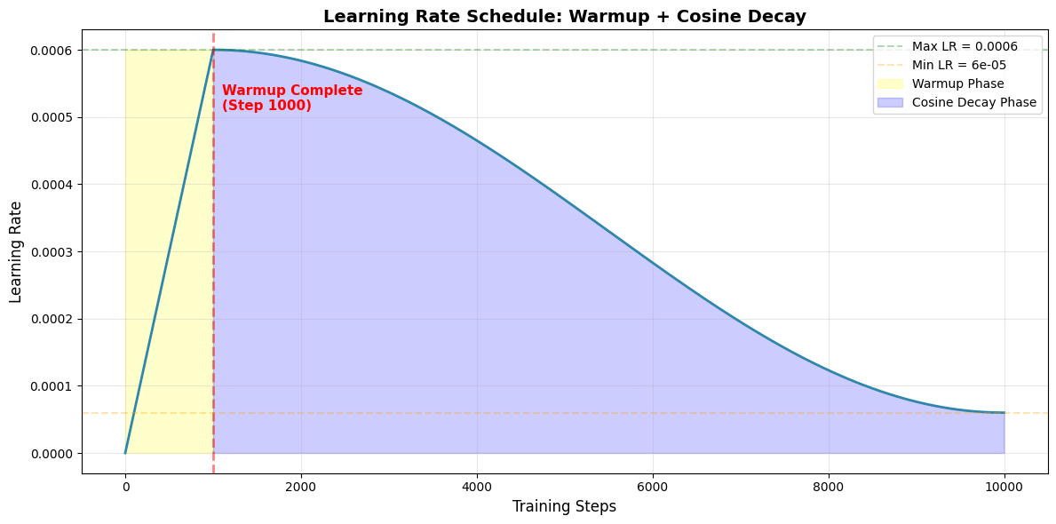
Why this pattern works:

• Warmup (yellow): Prevents large gradient updates with random weights early on

• Peak (1000-2000 steps): Maximum learning happens when gradients are reliable

• Decay (blue): Gradually reduces learning rate for fine-tuning near optimal weights

Batch Size and Gradient Accumulation¶

Training LLMs requires processing lots of tokens. But GPU memory is limited.

The Problem:

• Ideal: batch_size = 512 (process 512 sequences at once)

• Reality: GPU can only fit batch_size = 8

The Solution: Gradient Accumulation

accumulation_steps = 64  # Effective batch = 8 * 64 = 512

optimizer.zero_grad()
for i, (x, y) in enumerate(train_loader):
    logits = model(x)
    loss = F.cross_entropy(logits.view(-1, vocab_size), y.view(-1))
    loss = loss / accumulation_steps  # Scale the loss
    loss.backward()  # Accumulate gradients

    if (i + 1) % accumulation_steps == 0:
        optimizer.step()  # Update weights
        optimizer.zero_grad()  # Reset gradients

How it works:

1. Process small batches (8 sequences)

2. Accumulate gradients over 64 small batches

3. Update weights once using the accumulated gradient (equivalent to batch=512)

Benefits:

• Train with large effective batch sizes on limited hardware

• More stable gradients (averaging over more examples)

• Same results as true large batches, just slower

Summary¶

1. Self-Supervision: The model teaches itself by using the next word in a text as its own target.

2. The Loss Function: Cross-Entropy penalizes the model for being “surprised” by the correct word. A loss of 2.0 means perplexity ~7, indicating confusion between 7-8 likely tokens.

3. Optimization: We use the gradient of the loss to adjust the millions of parameters in our Attention heads and Feed-Forward layers.

4. Learning Rate Scheduling: Warmup and cosine decay help stabilize training and improve final performance.

5. Gradient Accumulation: Enables training with large effective batch sizes despite memory constraints.

Next Up: L09 – Inference & Sampling. Now that we have a trained brain, how do we actually get it to “talk” to us? We’ll learn about Temperature, Top-K, and Top-P sampling to control the model’s creativity.