L03 - Self-Attention: The Search Engine of Language
Building the “brain” of the Transformer: How words talk to each other.
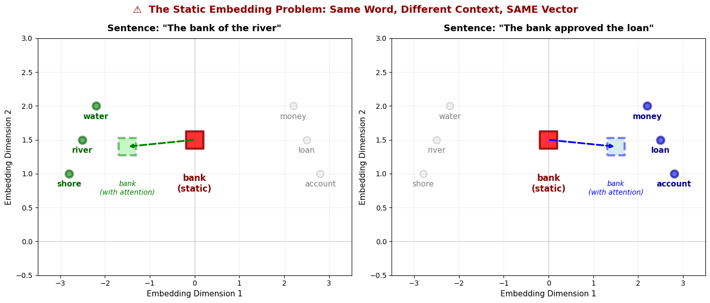
In L02 - Embeddings, we turned words into vectors and gave them positions. But there is still a fatal flaw: each word gets the same vector every time, regardless of context.
Consider the word “Bank”.
“The bank of the river.” (Nature)
“The bank approved the loan.” (Finance)
In a static embedding layer (a simple lookup table), the vector for “bank” is identical in both sentences. The model sees the same token ID → same vector, regardless of whether “bank” appears near “river” or “loan”.
import logging
import warnings

logging.getLogger("matplotlib.font_manager").setLevel(logging.ERROR)

import numpy as np
import matplotlib.pyplot as plt

# Create side-by-side comparison
fig, (ax1, ax2) = plt.subplots(1, 2, figsize=(14, 6))

# Define semantic clusters (same for both subplots)
nature_words = {'river': [-2.5, 1.5], 'water': [-2.2, 2.0], 'shore': [-2.8, 1.0]}
finance_words = {'loan': [2.5, 1.5], 'money': [2.2, 2.0], 'account': [2.8, 1.0]}

# Static embedding position for "bank" (same in both contexts!)
bank_static_pos = [0, 1.5]

# Where "bank" SHOULD move with attention
bank_nature_pos = [-1.5, 1.4]   # Shifted toward nature cluster
bank_finance_pos = [1.5, 1.4]   # Shifted toward finance cluster

# --- LEFT PLOT: "The bank of the river" ---
ax1.set_title('Sentence: "The bank of the river"', fontsize=13, fontweight='bold', pad=10)

# Plot nature cluster (highlighted with thicker border)
for word, pos in nature_words.items():
    ax1.scatter(pos[0], pos[1], c='green', s=100, alpha=0.6, edgecolors='darkgreen', linewidth=3, zorder=2)
    ax1.text(pos[0], pos[1]-0.1, word, ha='center', va='top', fontsize=11, fontweight='bold', color='darkgreen')

# Plot finance cluster (faded)
for word, pos in finance_words.items():
    ax1.scatter(pos[0], pos[1], c='lightgray', s=100, alpha=0.3, edgecolors='gray', linewidth=1.5, zorder=1)
    ax1.text(pos[0], pos[1]-0.1, word, ha='center', va='top', fontsize=11, color='gray')

# Static "bank" (red, same position as right plot)
ax1.scatter(bank_static_pos[0], bank_static_pos[1], c='red', s=600, alpha=0.8,
           edgecolors='darkred', linewidth=3, zorder=3, marker='s')
ax1.text(bank_static_pos[0], bank_static_pos[1]-0.5, 'bank\n(static)', ha='center', va='top',
        fontsize=12, fontweight='bold', color='darkred')

# Where it SHOULD be with attention (green ghost)
ax1.scatter(bank_nature_pos[0], bank_nature_pos[1], c='lightgreen', s=600, alpha=0.5,
           edgecolors='green', linewidth=3, linestyle='--', zorder=2, marker='s')
ax1.text(bank_nature_pos[0], bank_nature_pos[1]-0.5, 'bank\n(with attention)', ha='center', va='top',
        fontsize=10, color='green', style='italic')

# Arrow showing desired shift
ax1.annotate('', xy=bank_nature_pos, xytext=bank_static_pos,
            arrowprops=dict(arrowstyle='->', color='green', lw=2.5, linestyle='dashed'))

ax1.set_xlim(-3.5, 3.5)
ax1.set_ylim(-0.5, 3)
ax1.set_xlabel('Embedding Dimension 1', fontsize=11)
ax1.set_ylabel('Embedding Dimension 2', fontsize=11)
ax1.grid(True, alpha=0.2)
ax1.axhline(y=0, color='k', linewidth=0.5, alpha=0.3)
ax1.axvline(x=0, color='k', linewidth=0.5, alpha=0.3)

# --- RIGHT PLOT: "The bank approved the loan" ---
ax2.set_title('Sentence: "The bank approved the loan"', fontsize=13, fontweight='bold', pad=10)

# Plot finance cluster (highlighted)
for word, pos in finance_words.items():
    ax2.scatter(pos[0], pos[1], c='blue', s=100, alpha=0.6, edgecolors='darkblue', linewidth=3, zorder=2)
    ax2.text(pos[0], pos[1]-0.1, word, ha='center', va='top', fontsize=11, fontweight='bold', color='darkblue')

# Plot nature cluster (faded)
for word, pos in nature_words.items():
    ax2.scatter(pos[0], pos[1], c='lightgray', s=100, alpha=0.3, edgecolors='gray', linewidth=1.5, zorder=1)
    ax2.text(pos[0], pos[1]-0.1, word, ha='center', va='top', fontsize=11, color='gray')

# Static "bank" (red, SAME position as left plot!)
ax2.scatter(bank_static_pos[0], bank_static_pos[1], c='red', s=600, alpha=0.8,
           edgecolors='darkred', linewidth=3, zorder=3, marker='s')
ax2.text(bank_static_pos[0], bank_static_pos[1]-0.5, 'bank\n(static)', ha='center', va='top',
        fontsize=12, fontweight='bold', color='darkred')

# Where it SHOULD be with attention (blue ghost)
ax2.scatter(bank_finance_pos[0], bank_finance_pos[1], c='lightblue', s=600, alpha=0.5,
           edgecolors='blue', linewidth=3, linestyle='--', zorder=2, marker='s')
ax2.text(bank_finance_pos[0], bank_finance_pos[1]-0.5, 'bank\n(with attention)', ha='center', va='top',
        fontsize=10, color='blue', style='italic')

# Arrow showing desired shift
ax2.annotate('', xy=bank_finance_pos, xytext=bank_static_pos,
            arrowprops=dict(arrowstyle='->', color='blue', lw=2.5, linestyle='dashed'))

ax2.set_xlim(-3.5, 3.5)
ax2.set_ylim(-0.5, 3)
ax2.set_xlabel('Embedding Dimension 1', fontsize=11)
ax2.set_ylabel('Embedding Dimension 2', fontsize=11)
ax2.grid(True, alpha=0.2)
ax2.axhline(y=0, color='k', linewidth=0.5, alpha=0.3)
ax2.axvline(x=0, color='k', linewidth=0.5, alpha=0.3)

# Overall title
fig.suptitle('⚠️  The Static Embedding Problem: Same Word, Different Context, SAME Vector',
            fontsize=14, fontweight='bold', color='darkred', y=0.98)

plt.tight_layout()
plt.show()
The Problem Visualized:
Notice the red square labeled “bank (static)” is at the EXACT SAME POSITION in both plots. Whether “bank” appears in a sentence about rivers or loans, the static embedding lookup table returns the identical vector.
What We Need (shown by dashed arrows):
Left: In “The bank of the river”, we want “bank” to shift toward the nature cluster (green)
Right: In “The bank approved the loan”, we want “bank” to shift toward the finance cluster (blue)
Self-Attention is the mechanism that enables this context-dependent shift—it allows “bank” to dynamically adjust its representation based on surrounding words.
By the end of this post, you’ll understand:
The Query, Key, Value analogy (it’s just a database lookup!).
Why we need to scale our dot products (fixing the “magnitude” bug).
How to implement the famous attention equation from scratch.
We’ve seen that static embeddings give “bank” the same vector whether it appears with “river” or “loan”. How does attention fix this? It allows each word to look at its neighbors and adjust its meaning based on what it finds.
The math of Attention can look scary, but the concept is simple. It is a Soft Database Lookup.
Let’s trace how “bank” would use attention to shift its meaning in “The bank of the river”:
“bank” generates its Query: “What context am I in?”
It compares this Query against every other word’s Key:
“river” Key: “I’m a geographic feature” → High match!
“of” Key: “I’m a preposition” → Low match
“the” Key: “I’m an article” → Low match
“bank” finds the highest match with “river”
It extracts the Value from “river” (its semantic meaning) and adds it to its own representation
Now, the vector for “bank” is no longer just the static embedding; it is “bank + a lot of ‘river’ + a little bit of ‘the’ and ‘of’”. The representation has shifted toward the nature/geography meaning!
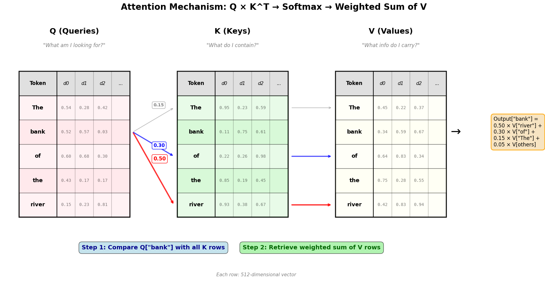
Here’s this process visualized. The diagram shows the complete attention computation: Q × K^T → Softmax → Weighted Sum of V. Notice how “bank” attends most strongly to “river” (0.50 weight), which disambiguates it toward the geographical meaning!
import matplotlib.pyplot as plt
import matplotlib.patches as mpatches
from matplotlib.patches import FancyArrowPatch
import numpy as np

def visualize_qkv_tables_with_arrows():
    """
    Show Q, K, V as proper tables with grid lines and column headers
    """
    tokens = ["The", "bank", "of", "the", "river"]
    seq_len = len(tokens)

    fig, ax = plt.subplots(1, 1, figsize=(18, 10))
    ax.set_xlim(0, 16)
    ax.set_ylim(-2.5, seq_len + 3)
    ax.axis('off')

    # Positions for the three tables
    q_x, k_x, v_x = 0.5, 5.5, 10.5
    table_width = 3.5
    row_height = 0.9

    # Helper function to draw a table
    def draw_table(x, y_start, title, color, num_cols=4, table_seed=0):
        # Title
        ax.text(x + table_width/2, y_start + seq_len + 1.8, title,
                fontsize=18, fontweight='bold', ha='center')

        # Subtitle
        subtitles = {
            'Q (Queries)': '"What am I looking for?"',
            'K (Keys)': '"What do I contain?"',
            'V (Values)': '"What info do I carry?"'
        }
        ax.text(x + table_width/2, y_start + seq_len + 1.3, subtitles.get(title, ''),
                fontsize=12, ha='center', style='italic', color='gray')

        # Table border
        border = mpatches.Rectangle((x, y_start), table_width, seq_len * row_height + row_height,
                                   linewidth=2.5,
                                   edgecolor='black',
                                   facecolor='none')
        ax.add_patch(border)

        # Column headers
        header_y = y_start + seq_len * row_height
        header_rect = mpatches.Rectangle((x, header_y), table_width, row_height,
                                        linewidth=2,
                                        edgecolor='black',
                                        facecolor='lightgray',
                                        alpha=0.7)
        ax.add_patch(header_rect)

        # Token column header
        ax.text(x + 0.6, header_y + row_height/2, 'Token',
               fontsize=12, fontweight='bold', ha='center', va='center')

        # Dimension columns header
        col_width = (table_width - 1.2) / num_cols
        for i in range(num_cols):
            col_x = x + 1.2 + i * col_width
            ax.text(col_x + col_width/2, header_y + row_height/2,
                   f'd{i}' if i < 3 else '...',
                   fontsize=11, ha='center', va='center', style='italic')
            # Vertical grid line
            if i > 0:
                ax.plot([col_x, col_x], [y_start, header_y + row_height],
                       'k-', linewidth=1, alpha=0.3)

        # Draw rows
        for i, token in enumerate(tokens):
            y = y_start + (seq_len - i - 1) * row_height

            # Row background (alternating)
            row_rect = mpatches.Rectangle((x, y), table_width, row_height,
                                         linewidth=1,
                                         edgecolor='black',
                                         facecolor=color,
                                         alpha=0.2 if i % 2 == 0 else 0.35)
            ax.add_patch(row_rect)

            # Horizontal grid line
            ax.plot([x, x + table_width], [y, y], 'k-', linewidth=1, alpha=0.3)

            # Token label (first column)
            ax.text(x + 0.6, y + row_height/2, token,
                   fontsize=13, fontweight='bold', ha='center', va='center')

            # Vertical separator after token column
            ax.plot([x + 1.2, x + 1.2], [y_start, header_y + row_height],
                   'k-', linewidth=1.5, alpha=0.5)

            # Dummy values in cells - different for each table
            np.random.seed(table_seed * 100 + i)  # Different seed per table and row
            for j in range(num_cols):
                col_x = x + 1.2 + j * col_width
                if j < 3:
                    val = np.random.rand()
                    ax.text(col_x + col_width/2, y + row_height/2,
                           f'{val:.2f}',
                           fontsize=10, ha='center', va='center',
                           alpha=0.5, family='monospace')

        return y_start + seq_len * row_height / 2  # Return center y position

    # Draw the three tables
    y_start = 0.5
    q_center_y = draw_table(q_x, y_start, 'Q (Queries)', 'pink', num_cols=4, table_seed=1)
    k_center_y = draw_table(k_x, y_start, 'K (Keys)', 'lightgreen', num_cols=4, table_seed=2)
    v_center_y = draw_table(v_x, y_start, 'V (Values)', 'lightyellow', num_cols=4, table_seed=3)

    # Example: "bank" attending to tokens
    bank_idx = 1
    bank_y = y_start + (seq_len - bank_idx - 1) * row_height + row_height/2

    # Arrow from Q["bank"] to all K
    # Q["bank"] → K["river"] (strongest - disambiguates to geography meaning)
    river_idx = 4
    river_y = y_start + (seq_len - river_idx - 1) * row_height + row_height/2
    arrow_label_x = (q_x + table_width + k_x)/2

    ax.annotate('', xy=(k_x - 0.1, river_y), xytext=(q_x + table_width + 0.1, bank_y),
                arrowprops=dict(arrowstyle='->', lw=3, color='red', alpha=0.8))
    ax.text(arrow_label_x, (bank_y + river_y)/2 + 0.3, '0.50',
            fontsize=12, color='red', fontweight='bold',
            bbox=dict(boxstyle='round,pad=0.3', facecolor='white', edgecolor='red'))

    # Q["bank"] → K["of"] (preposition - moderate relevance)
    of_idx = 2
    of_y = y_start + (seq_len - of_idx - 1) * row_height + row_height/2
    ax.annotate('', xy=(k_x - 0.1, of_y), xytext=(q_x + table_width + 0.1, bank_y),
                arrowprops=dict(arrowstyle='->', lw=2.5, color='blue', alpha=0.7))
    ax.text(arrow_label_x, (bank_y + of_y)/2 - 0.1, '0.30',
            fontsize=11, color='blue', fontweight='bold',
            bbox=dict(boxstyle='round,pad=0.3', facecolor='white', edgecolor='blue'))

    # Q["bank"] → K["The"] (weaker - determiner)
    the_idx = 0
    the_y = y_start + (seq_len - the_idx - 1) * row_height + row_height/2
    ax.annotate('', xy=(k_x - 0.1, the_y), xytext=(q_x + table_width + 0.1, bank_y),
                arrowprops=dict(arrowstyle='->', lw=1.5, color='gray', alpha=0.5))
    ax.text(arrow_label_x, (bank_y + the_y)/2 + 0.5, '0.15',
            fontsize=10, color='gray', fontweight='bold',
            bbox=dict(boxstyle='round,pad=0.3', facecolor='white', edgecolor='gray', alpha=0.7))

    # After attention: K → V (the values that get retrieved)
    # K["river"] → V["river"]
    ax.annotate('', xy=(v_x - 0.1, river_y), xytext=(k_x + table_width + 0.1, river_y),
                arrowprops=dict(arrowstyle='->', lw=3, color='red', alpha=0.8))

    # K["of"] → V["of"]
    ax.annotate('', xy=(v_x - 0.1, of_y), xytext=(k_x + table_width + 0.1, of_y),
                arrowprops=dict(arrowstyle='->', lw=2.5, color='blue', alpha=0.7))

    # K["The"] → V["The"]
    ax.annotate('', xy=(v_x - 0.1, the_y), xytext=(k_x + table_width + 0.1, the_y),
                arrowprops=dict(arrowstyle='->', lw=1.5, color='gray', alpha=0.5))

    # Final output annotation
    output_y = bank_y
    ax.text(v_x + table_width + 0.3, output_y, '→', fontsize=29, ha='center', va='center')
    ax.text(v_x + table_width + 1.5, output_y,
            'Output["bank"] =\n0.50 × V["river"] +\n0.30 × V["of"] +\n0.15 × V["The"] +\n0.05 × V[others]',
            fontsize=12, ha='left', va='center',
            bbox=dict(boxstyle='round,pad=0.5', facecolor='wheat',
                     edgecolor='orange', linewidth=2, alpha=0.8))

    # Add step labels with background (below tables, above dimension annotation)
    step1_y = -0.7
    ax.text((q_x + k_x + table_width)/2, step1_y, r'Step 1: Compare Q["bank"] with all K rows',
            fontsize=14, ha='center', fontweight='bold', color='darkblue',
            bbox=dict(boxstyle='round,pad=0.5', facecolor='lightblue', alpha=0.7))

    ax.text((k_x + v_x + table_width)/2, step1_y, r'Step 2: Retrieve weighted sum of V rows',
            fontsize=14, ha='center', fontweight='bold', color='darkgreen',
            bbox=dict(boxstyle='round,pad=0.5', facecolor='lightgreen', alpha=0.7))

    # Main title
    plt.suptitle('Attention Mechanism: Q × K^T → Softmax → Weighted Sum of V',
                 fontsize=20, fontweight='bold', y=0.98)

    # Add dimension annotation
    ax.text(8, -1.7, 'Each row: 512-dimensional vector',
            fontsize=11, ha='center', style='italic', color='gray')

    plt.tight_layout()
    return fig

# Create and save the visualization
fig = visualize_qkv_tables_with_arrows()
plt.show()
Key Insights from the Visualization:
Q, K, V are Tables: Each has one row per token, with columns representing dimensions (typically 512 in real transformers, though we show just a few here for clarity).
Query-Key Matching (Step 1): When “bank” (the query token) wants to understand its context, it compares its Query vector Q[“bank”] against ALL Key vectors. The comparison produces attention scores:
Q[“bank”] · K[“river”] = 0.50 (highest: disambiguates to geographical meaning!)
Retrieve Values (Step 2): These scores become weights that determine how much of each Value vector to retrieve. The final output for “bank” is a weighted combination: primarily V[“river”] (50%), with contributions from V[“of”] (30%) and other tokens. This shifts “bank” toward its geographical meaning!
Real Dimensions: While we show 3-4 dimensions for clarity, real transformers use 512 or more dimensions, allowing for much richer semantic relationships.
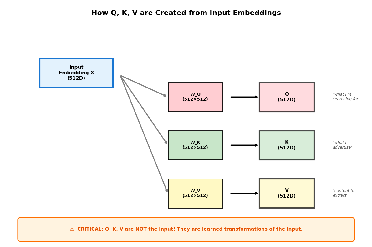
In the visualization above, we showed Q, K, V as three separate tables. But where do these tables come from? A critical point that’s often misunderstood:
Let’s visualize how these projections work:
import matplotlib.pyplot as plt
import matplotlib.patches as patches

fig, ax = plt.subplots(figsize=(12, 8))
ax.set_xlim(0, 10)
ax.set_ylim(0, 10)
ax.axis('off')

# Title
ax.text(5, 9.5, 'How Q, K, V are Created from Input Embeddings',
        ha='center', fontsize=16, fontweight='bold')

# Input embedding box
input_box = patches.Rectangle((1, 6.5), 2, 1.2,
                               facecolor='#e3f2fd', edgecolor='#1976d2', linewidth=3)
ax.add_patch(input_box)
ax.text(2, 7.1, 'Input\nEmbedding X\n(512D)', ha='center', va='center',
        fontsize=11, fontweight='bold')

# Projection matrices
matrices_y = [5.5, 3.5, 1.5]
colors = ['#ffcdd2', '#c8e6c9', '#fff9c4']
labels = ['W_Q', 'W_K', 'W_V']
outputs = ['Q', 'K', 'V']
descriptions = [
    '"what I\'m\nsearching for"',
    '"what I\nadvertise"',
    '"content to\nextract"'
]

for i, (y, color, label, output, desc) in enumerate(zip(matrices_y, colors, labels, outputs, descriptions)):
    # Arrow from input to matrix
    ax.annotate('', xy=(4.5, y + 0.6), xytext=(3.2, 7.0),
                arrowprops=dict(arrowstyle='->', lw=2.5, color='gray'))

    # Matrix box
    matrix_box = patches.Rectangle((4.5, y), 1.5, 1.2,
                                   facecolor=color, edgecolor='black', linewidth=2)
    ax.add_patch(matrix_box)
    ax.text(5.25, y + 0.6, f'{label}\n(512×512)', ha='center', va='center',
            fontsize=10, fontweight='bold')

    # Arrow from matrix to output
    ax.annotate('', xy=(7, y + 0.6), xytext=(6.2, y + 0.6),
                arrowprops=dict(arrowstyle='->', lw=2.5, color='black'))

    # Output box
    output_box = patches.Rectangle((7, y), 1.5, 1.2,
                                   facecolor=color, edgecolor='black', linewidth=3, alpha=0.7)
    ax.add_patch(output_box)
    ax.text(7.75, y + 0.6, f'{output}\n(512D)', ha='center', va='center',
            fontsize=11, fontweight='bold')

    # Description
    ax.text(9, y + 0.6, desc, ha='left', va='center',
            fontsize=9, style='italic', color='#555')

# Key insight box at bottom
insight_box = patches.FancyBboxPatch((0.5, 0.2), 9, 0.8,
                                     boxstyle="round,pad=0.1",
                                     facecolor='#fff3e0', edgecolor='#ff6f00', linewidth=2)
ax.add_patch(insight_box)
ax.text(5, 0.6, '⚠️  CRITICAL: Q, K, V are NOT the input! They are learned transformations of the input.',
        ha='center', va='center', fontsize=11, fontweight='bold', color='#e65100')

plt.tight_layout()
plt.show()
Now let’s see this in code:
# REALITY: Q, K, V come from learned projections of the embeddings
import torch

# Input: embeddings for "bank", "river", "loan"
# Static embeddings (in reality, these would come from the embedding layer)
bank_embedding = torch.tensor([0.5, 0.3, 0.8, 0.2])
river_embedding = torch.tensor([0.2, 0.9, 0.1, 0.3])
loan_embedding = torch.tensor([0.8, 0.1, 0.4, 0.7])

embeddings = torch.stack([bank_embedding, river_embedding, loan_embedding])  # [3, 4]
print("Input embeddings [3 tokens, 4 dims]:")
print(embeddings)
print()

# Learned projection matrices (in real models, these are trained)
# For this demo, we'll create random matrices
torch.manual_seed(42)
d_model = 4  # embedding dimension
W_Q = torch.randn(d_model, d_model) * 0.5  # [4, 4]
W_K = torch.randn(d_model, d_model) * 0.5  # [4, 4]
W_V = torch.randn(d_model, d_model) * 0.5  # [4, 4]

# Project embeddings to Q, K, V
Q = embeddings @ W_Q  # [3, 4] @ [4, 4] = [3, 4]
K = embeddings @ W_K  # [3, 4]
V = embeddings @ W_V  # [3, 4]

print("After learned projections:")
print(f"  Q shape: {Q.shape}  (each embedding transformed by W_Q)")
print(f"  K shape: {K.shape}  (each embedding transformed by W_K)")
print(f"  V shape: {V.shape}  (each embedding transformed by W_V)")
print()
print("Q (queries):")
print(Q)
print()
print("Notice: Q is DIFFERENT from the input embeddings!")
print("The projection matrices mixed and transformed the original features.")
Input embeddings [3 tokens, 4 dims]:
tensor([[0.5000, 0.3000, 0.8000, 0.2000],
        [0.2000, 0.9000, 0.1000, 0.3000],
        [0.8000, 0.1000, 0.4000, 0.7000]])

After learned projections:
  Q shape: torch.Size([3, 4])  (each embedding transformed by W_Q)
  K shape: torch.Size([3, 4])  (each embedding transformed by W_K)
  V shape: torch.Size([3, 4])  (each embedding transformed by W_V)

Q (queries):
tensor([[ 0.2098,  0.7902, -0.0152, -1.2523],
        [ 0.3512, -0.4083, -0.0643, -0.8885],
        [ 0.3995,  0.6671,  0.0105, -0.9363]])

Notice: Q is DIFFERENT from the input embeddings!
The projection matrices mixed and transformed the original features.
Remember from L02: “The attention mechanism is parallel. It looks at every word in a sentence at the exact same time.”
This is the breakthrough that makes Transformers faster AND better at understanding language than older architectures like RNNs (Recurrent Neural Networks).
How RNNs Process a Sentence (Sequential):
RNNs maintain a “hidden state”—a vector that accumulates information from all previous words. At each step, the hidden state combines the current word with everything seen so far.
Let’s trace a concrete example: pronoun resolution. When the model processes “it”, how does it figure out that “it” refers to “bank”? We’ll follow how information flows through the hidden states.
Input: "The bank approved the loan because it was well-capitalized"
        ↑    ↑                              ↑
      word 1  word 2                       word 7

Step 1: "The"      → hidden_state_1 = f(embedding("The"))
                      ↓ Contains: [info about "The"]

Step 2: "bank"     → hidden_state_2 = f(embedding("bank"), hidden_state_1)
                      ↓ Contains: [info about "The", "bank"] compressed into one vector

Step 3: "approved" → hidden_state_3 = f(embedding("approved"), hidden_state_2)
                      ↓ Contains: [info about "The", "bank", "approved"] compressed

...

Step 7: "it"       → hidden_state_7 = f(embedding("it"), hidden_state_6)
                      ↓ Contains: [ALL 7 words] compressed into a fixed-size vector

Problem: To understand what "it" refers to, information about "bank" (word 2)
must pass through a chain of compressions before reaching "it" (word 7):

  hidden_state_2 (contains "bank" info)
    ↓ compressed with "approved"
  hidden_state_3
    ↓ compressed with "the"
  hidden_state_4
    ↓ compressed with "loan"
  hidden_state_5
    ↓ compressed with "because"
  hidden_state_6 (used by "it" at step 7)

Information about "bank" has been compressed through 4 intermediate mixing steps.
The more steps between "bank" and "it", the more diluted the information becomes.
This is the "vanishing gradient" problem (where gradient signals become too small to effectively update earlier layers during backpropagation).

Total: 7 sequential steps (MUST run one-by-one)
The Hidden State Bottleneck:
The hidden state is accumulative (it tries to remember everything), but it achieves this through compression into a fixed-size vector (typically 512 or 1024 dimensions).
Think of it like this: After reading “The bank approved the loan because it”, the RNN must squeeze all understanding of these 7 words—their meanings, relationships, syntactic roles—into a single vector of fixed size. Then it must use this compressed summary to process “was” and “well-capitalized”.
It’s like trying to fit an entire Wikipedia article into a tweet, then using only that tweet to write the next paragraph. Some information inevitably gets lost or diluted.
How Attention Processes the Same Sentence (Parallel):
Now let’s see how attention solves the same pronoun resolution task: when “it” needs to figure out what it refers to.
Instead of passing information through a chain of hidden states, attention allows direct connections between any two words.
Input: "The bank approved the loan because it was well-capitalized"

Single Step: ALL words computed simultaneously via matrix operations:

"it" (word 7) compares its Query directly against ALL Keys:
  Q("it") · K("The")      = 0.05  → Low attention weight
  Q("it") · K("bank")     = 0.82  → HIGH attention weight! ✓
  Q("it") · K("approved") = 0.08  → Low attention weight
  Q("it") · K("the")      = 0.02  → Low attention weight
  Q("it") · K("loan")     = 0.15  → Medium attention weight
  ...

Result: "it" can look DIRECTLY at "bank" (word 2) without any intermediate recurrent steps.
No repeated hidden-state bottleneck — just one parallel compare-and-mix step per layer.

Every other word does the same computation simultaneously:
  - "The" attends to all words
  - "bank" attends to all words
  - "approved" attends to all words
  ... (all computed in parallel)

Total: 1 parallel step (all comparisons at once, then weighted sum)
Why Direct Access Matters:
No information loss: “it” doesn’t need to hope that information about “bank” survived 4 intermediate compressions (hidden states 3→4→5→6)
Long-range dependencies: Works just as well for word 100 referring to word 1 as for adjacent words
Symmetry: “bank” can attend to “loan” just as easily as “loan” attends to “bank”
Multiple relationships: Each word can attend strongly to multiple other words simultaneously (through the weighted sum)
Concrete Example – Pronoun Resolution (soft, not magic):
Consider: “The artist gave the musician a score because she loved her composition.”
This sentence is genuinely ambiguous: humans can reasonably map “she/her” to either person depending on how they interpret “score/composition”.
RNN: By the time we reach “she”, the model has compressed everything so far into one hidden state, which can make it harder to keep distinct candidates (“artist” vs “musician”) separable over long distances.
Attention: “she” compares its Query against all Keys directly and produces a weighting over candidates. If the context provides a strong cue, attention can put more weight on the best-fitting antecedent; if the context is symmetric, weights may stay split and later layers may or may not sharpen the preference.
Why This Works:
The attention mechanism achieves parallelism through matrix multiplication. When we compute QKT (which you’ll see shortly), we’re not looping through words one-by-one. Instead:
Every word generates its Query, Key, and Value simultaneously (one matrix operation)
Every Query compares against every Key simultaneously (another matrix operation)
Every word gets its context-aware representation simultaneously (final matrix operation)
Modern GPUs are optimized for matrix operations, so computing attention for 100 words in parallel is barely slower than computing it for 10 words. This is why Transformers can handle such long contexts efficiently.
Now let’s see the math that makes this parallelism possible.
In Part 1, we saw the intuition behind Q/K/V. In Part 2, we learned these are learned projections. In Part 3, we explored parallelism. Now let’s dive into the math: How do we “compare” two vectors? How do we measure if a Query is similar to a Key?
The answer: the Dot Product.
The dot product is a mathematical operation that measures alignment between two vectors. If two vectors point in the same direction, the result is large and positive. If they point in opposite directions, it is negative. If they’re perpendicular, the result is zero.
This is how attention computes “relevance”: Q(“it”) · K(“bank”) gives us a score measuring how much “it” should attend to “bank”.
However, there is a catch. The dot product captures both alignment and magnitude. Before we look at the formula, let’s visualize why this is dangerous for neural networks.
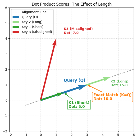
In the plot below, we compare a Query (Blue) against three different Keys.
K1 (Short): Perfectly aligned with Q, but small.
K2 (Long): Perfectly aligned with Q, but large.
K3 (Misaligned): Pointing in a different direction.
First, let’s compute the scores numerically to see the problem:
# Computing dot products to measure similarity
import torch

Q = torch.tensor([3.0, 1.0])
K1_short = torch.tensor([1.5, 0.5])
K2_long = torch.tensor([4.5, 1.5])
K3_misaligned = torch.tensor([1.0, 4.0])

print("🎯 Dot Product Scores:")
print(f"  K1 (short, aligned):     {torch.dot(Q, K1_short):.1f}")
print(f"  K2 (long, aligned):      {torch.dot(Q, K2_long):.1f}")
print(f"  K3 (misaligned):         {torch.dot(Q, K3_misaligned):.1f}")
print(f"\n⚠️  K3 (misaligned) scores higher than K1 (aligned)!")
print(f"     This is the magnitude problem we need to fix with scaling.")
🎯 Dot Product Scores:
  K1 (short, aligned):     5.0
  K2 (long, aligned):      15.0
  K3 (misaligned):         7.0

⚠️  K3 (misaligned) scores higher than K1 (aligned)!
     This is the magnitude problem we need to fix with scaling.
Why this is a problem:
Look at the score for K3 (Misaligned). It scored 7.0.
Now look at K1 (Short). It scored 5.0.
The “Misaligned” vector beat the “Perfectly Aligned” vector simply because it was longer. If we don’t fix this, our model will prioritize “loud” signals (large numbers) over “correct” signals (aligned meaning).
We fix this by Scaling: we divide the result by the square root of the dimension (dk), where dk is the dimensionality of the Q and K vectors. This normalizes the scores so the model focuses on alignment, not magnitude.
Let’s see scaling in action with a concrete example:
# Why scaling matters: A concrete example
import torch

Q = torch.tensor([3.0, 1.0])
K_aligned = torch.tensor([3.0, 1.0])
K_misaligned = torch.tensor([1.0, 4.0])

score_aligned = torch.dot(Q, K_aligned)
score_misaligned = torch.dot(Q, K_misaligned)

print("Without Scaling:")
print(f"  Aligned score:     {score_aligned:.1f}")
print(f"  Misaligned score:  {score_misaligned:.1f}")
print(f"  Ratio:             {score_aligned/score_misaligned:.2f}x\n")

# Apply scaling
d_k = 2  # Dimensionality of Q and K vectors (both are 2D in this example)
scaled_aligned = score_aligned / torch.sqrt(torch.tensor(d_k, dtype=torch.float32))
scaled_misaligned = score_misaligned / torch.sqrt(torch.tensor(d_k, dtype=torch.float32))

print("With Scaling (÷√2 ≈ ÷1.41):")
print(f"  Aligned score:     {scaled_aligned:.2f}")
print(f"  Misaligned score:  {scaled_misaligned:.2f}")
print(f"  Ratio:             {scaled_aligned/scaled_misaligned:.2f}x")
print(f"\n✓ The ratio stays the same, but values are controlled")
Without Scaling:
  Aligned score:     10.0
  Misaligned score:  7.0
  Ratio:             1.43x

With Scaling (÷√2 ≈ ÷1.41):
  Aligned score:     7.07
  Misaligned score:  4.95
  Ratio:             1.43x

✓ The ratio stays the same, but values are controlled
The Scores (QKT): We multiply the Query of the current word by the Keys of all words. (The T superscript means “transpose”—we flip rows and columns of the K matrix so the dimensions align for multiplication.)
The Scaling (dk): We shrink the scores by dividing by dk (where dk is the dimension of the Q and K vectors) to prevent exploding values.
Softmax (The Probability): We convert scores into probabilities that sum to 1.0.
The Weighted Sum (V): We multiply the probabilities by the Values to get the final context vector.
Let’s trace the math using vectors from the plot above. We’ll use the pronoun resolution example: when “it” (query) attends to “animal”, “street”, and “because” (keys). Note that we’re reusing the same Q=[3,1] vector from the magnitude visualization—now applying it to a concrete language example.
Recall that:
Q (Query): What “it” is looking for (its search query)
K (Keys): What each word advertises about itself (folder labels)
V (Values): The actual semantic content to extract (the documents inside)
Inputs:
Query (Q):[3, 1]
Keys:
K_animal (Exact Match):[3, 1]
K_street (Misaligned):[1, 4]
K_because (Short, aligned):[1.5, 0.5]
Values:
V_animal:[2.0, 1.5]
V_street:[0.5, 0.3]
V_because:[-0.5, 1.2]
Let’s compute all four steps in executable code:
import torch
import torch.nn.functional as F

# Inputs
Q = torch.tensor([3.0, 1.0])
K = {
    'animal': torch.tensor([3.0, 1.0]),
    'street': torch.tensor([1.0, 4.0]),
    'because': torch.tensor([1.5, 0.5])
}
V = {
    'animal': torch.tensor([2.0, 1.5]),
    'street': torch.tensor([0.5, 0.3]),
    'because': torch.tensor([-0.5, 1.2])
}

print("Step 1: Compute Dot Products (Raw Scores)")
scores = {name: torch.dot(Q, k).item() for name, k in K.items()}
for name, score in scores.items():
    print(f"  {name:8s}: {score:.1f}")

print("\nStep 2: Scale by √d_k")
d_k = 2  # Dimensionality of Q and K (both are 2D in this example)
scaled = {name: score / torch.sqrt(torch.tensor(d_k)).item() for name, score in scores.items()}
for name, score in scaled.items():
    print(f"  {name:8s}: {score:.2f}")

print("\nStep 3: Softmax (Convert to Probabilities)")
scaled_tensor = torch.tensor(list(scaled.values()))
weights_tensor = F.softmax(scaled_tensor, dim=0)

for name, weight in zip(K.keys(), weights_tensor):
    print(f"  {name:8s}: {weight:.2f} ({weight*100:.0f}%)")

print("\nStep 4: Weighted Sum (Combine Values)")
V_stacked = torch.stack([V[name] for name in K.keys()])
context = torch.sum(weights_tensor.unsqueeze(1) * V_stacked, dim=0)
print(f"  Final context vector: [{context[0]:.2f}, {context[1]:.2f}]")
print(f"\n✓ Context is dominated by 'animal' (87% weight)")
Step 1: Compute Dot Products (Raw Scores)
  animal  : 10.0
  street  : 7.0
  because : 5.0

Step 2: Scale by √d_k
  animal  : 7.07
  street  : 4.95
  because : 3.54

Step 3: Softmax (Convert to Probabilities)
  animal  : 0.87 (87%)
  street  : 0.10 (10%)
  because : 0.03 (3%)

Step 4: Weighted Sum (Combine Values)
  Final context vector: [1.78, 1.37]

✓ Context is dominated by 'animal' (87% weight)
Now let’s walk through each step in detail:
Step 1: The Dot Product (QKT) - Computing Raw Scores
Score (animal): (3×3)+(1×1)=10
Score (street): (3×1)+(1×4)=7
Score (because): (3×1.5)+(1×0.5)=5
Step 2: Scaling (dk)
We divide by 2≈1.41.
Scaled Score (animal): 10/1.41≈7.09
Scaled Score (street): 7/1.41≈4.96
Scaled Score (because): 5/1.41≈3.54
Step 3: Softmax
We exponentiate and normalize to get percentages using the Softmax formula:
For a deeper dive into how softmax works, why we use exponentials, and numerical stability techniques, see our dedicated tutorial: Softmax: From Scores to Probabilities
Step 4: Weighted Sum (Combining Values)
Now we multiply each attention weight by its corresponding Value vector and sum them:
Notice how the mechanism successfully identified the aligned vector (“animal”) as the important one, giving it 87% of the attention weights (recall: weights are the post-softmax probabilities, while scores are the pre-softmax logits 7.09, 4.96, and 3.54). The final context vector [1.78, 1.37] is dominated by V_animal’s contribution, as we’ll see visualized below.
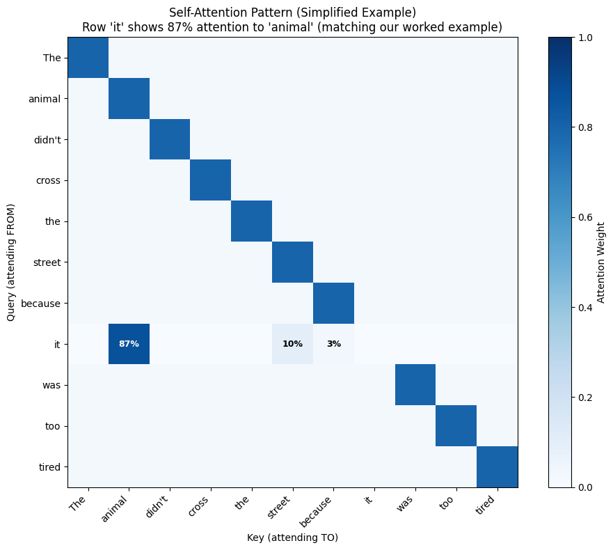
We’ve explored attention through different lenses—from the “bank” disambiguation problem to the worked example with pronoun resolution above. Now let’s see the full attention pattern for our pronoun resolution example as a heatmap.
In trained models, attention patterns emerge that capture semantic relationships. The heatmap below shows a simplified example to illustrate what we might expect: brighter colors represent higher attention weights (post-softmax probabilities).
import numpy as np
import matplotlib.pyplot as plt

# Simplified example: "The animal didn't cross the street because it was too tired"
# In a real model, "it" would ideally learn to attend to "animal" (not "street")
tokens = ["The", "animal", "didn't", "cross", "the", "street", "because", "it", "was", "too", "tired"]
data = np.zeros((len(tokens), len(tokens)))

it_idx = tokens.index("it")
animal_idx = tokens.index("animal")
street_idx = tokens.index("street")

# Matching our worked example: "it" attends to animal (87%), street (10%), because (3%)
because_idx = tokens.index("because")
data[it_idx, animal_idx] = 0.87  # Strong attention to "animal" (matches calculation)
data[it_idx, street_idx] = 0.10  # Weak attention to "street" (matches calculation)
data[it_idx, because_idx] = 0.03 # Very weak attention to "because" (matches calculation)

# Simple diagonal pattern for other words (attending to themselves)
for i in range(len(tokens)):
    if i != it_idx:
        data[i, i] = 0.8
        # Distribute remaining probability uniformly
        remaining = 0.2 / (len(tokens) - 1)
        for j in range(len(tokens)):
            if i != j:
                data[i, j] = remaining

plt.figure(figsize=(10, 8))
plt.imshow(data, cmap='Blues', vmin=0, vmax=1)
plt.xticks(range(len(tokens)), tokens, rotation=45, ha='right')
plt.yticks(range(len(tokens)), tokens)
plt.title("Self-Attention Pattern (Simplified Example)\nRow 'it' shows 87% attention to 'animal' (matching our worked example)")
plt.xlabel("Key (attending TO)")
plt.ylabel("Query (attending FROM)")
plt.colorbar(label='Attention Weight')

# Add text annotations for the "it" row to make it clearer
for j, token in enumerate(tokens):
    weight = data[it_idx, j]
    if weight > 0.02:  # Annotate weights from our worked example (87%, 10%, 3%)
        if abs(weight - 0.87) < 0.001: # Check for the 87% weight
            text_color = 'white'
        else:
            text_color = 'black'
        plt.text(j, it_idx, f'{weight:.0%}',
                ha='center', va='center', color=text_color, fontsize=9, fontweight='bold')

plt.tight_layout()
plt.show()
Before we implement the full attention class, let’s see how attention works with real tensors:
# Test attention mechanism step-by-step with PyTorch
import torch
import torch.nn.functional as F

# Create simple 3-token sequence with 4-dimensional embeddings
Q = torch.tensor([[3.0, 1.0, 0.0, 0.0],
                  [1.0, 4.0, 0.0, 0.0],
                  [2.0, 2.0, 0.0, 0.0]])  # [3 tokens, 4 dims]
K = Q.clone()  # For simplicity, keys = queries
V = torch.tensor([[1.0, 0.0, 0.0, 0.0],
                  [0.0, 1.0, 0.0, 0.0],
                  [0.5, 0.5, 0.0, 0.0]])  # [3 tokens, 4 dims]

d_k = Q.size(-1)  # Dimensionality of Q, K, and V (all are 4D here)

# Step by step
scores = torch.matmul(Q, K.T) / torch.sqrt(torch.tensor(d_k, dtype=torch.float32))
print("Scaled Scores (each token attending to all tokens):")
print(scores)
print()

weights = F.softmax(scores, dim=-1)
print("Attention Weights (after softmax):")
print(weights)
print(f"Row sums (should be 1.0): {weights.sum(dim=-1)}")
print()

output = torch.matmul(weights, V)
print("Output (context-aware representations):")
print(output)
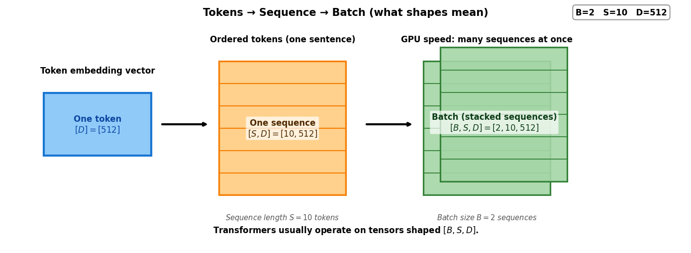
So far, we’ve worked with single sequences shaped [S, D] - one sentence at a time. In practice, we process multiple sequences simultaneously in a batch.
GPUs are designed for parallel computation. Processing 32 sequences takes roughly the same time as processing 1 sequence! This is why deep learning libraries operate on batches: [B, S, D] where:
B = Batch size (e.g., 32 sequences)
S = Sequence length (e.g., 10 tokens)
D = Embedding dimension (e.g., 512)
Here’s what “token”, “sequence”, and “batch” mean:
We’ve seen the intuition (Q/K/V database lookup), learned projections, parallelism, the math (dot products and scaling), visualization (attention heatmaps), and batching. Now let’s see how remarkably simple the actual code is.
We can implement this entire mechanism in fewer than 20 lines of code.
Note the use of masked_fill, which we will use in L06 - The Causal Mask to prevent the model from “cheating” by looking at future words.
import torch
import torch.nn as nn
import math

class ScaledDotProductAttention(nn.Module):
    def __init__(self, d_k):
        super().__init__()
        self.d_k = d_k  # Dimensionality of Q, K, and V vectors

    def forward(self, q, k, v, mask=None):
        # 1. Calculate the Dot Product (Scores)
        # q: [batch, seq, d_k]
        # k: [batch, seq, d_k]
        # v: [batch, seq, d_k]
        # scores shape: [batch, seq, seq]
        # Scale by sqrt(d_k) where d_k is the dimensionality of Q, K, and V
        scores = torch.matmul(q, k.transpose(-2, -1)) / math.sqrt(self.d_k)

        # 2. Apply Mask (Optional - vital for GPT!)
        if mask is not None:
            # We use a very large negative number so Softmax turns it to zero
            scores = scores.masked_fill(mask == 0, -1e9)

        # 3. Softmax to get probabilities (0.0 to 1.0)
        attn_weights = torch.softmax(scores, dim=-1)  # [batch, seq, seq]

        # 4. Multiply by Values to get the weighted context
        output = torch.matmul(attn_weights, v)  # [batch, seq, d_k]

        return output, attn_weights
Now let’s see how to use this class in practice. We need to create the projection layers and show the complete flow from embeddings to attention output:
import torch
import torch.nn as nn

# Example: Process a batch of 2 sequences, each with 10 tokens
# These values are intentionally small for demonstration purposes
batch_size = 2     # Small for demo (production: 8-512 depending on GPU memory)
seq_len = 10       # Short for demo (production: 128-2048+ depending on model)
d_model = 512      # Standard embedding dimension (used in BERT-base, GPT-2)
d_k = 64           # Dimensionality of Q, K, and V (= d_model / num_heads in multi-head)

# In production, hyperparameters are chosen based on:
# - batch_size: GPU memory constraints (larger = faster training but needs more VRAM)
# - seq_len: Task requirements (longer = more context but quadratic memory cost)
# - d_model: Model capacity (512 for base models, 768-1024 for large, 2048+ for XL)
# - d_k: Usually d_model / num_heads (e.g., 512 / 8 = 64 for 8-head attention)

# Step 1: Start with embeddings (normally from an embedding layer)
# Shape: [batch, seq, d_model]
embeddings = torch.randn(batch_size, seq_len, d_model)

# Step 2: Create the projection layers (learned during training)
# These transform embeddings into Q, K, V
W_q = nn.Linear(d_model, d_k, bias=False)
W_k = nn.Linear(d_model, d_k, bias=False)
W_v = nn.Linear(d_model, d_k, bias=False)

# Step 3: Project embeddings to create Q, K, V
# This is the X × W_Q, X × W_K, X × W_V we discussed earlier
# All three have the same dimensionality d_k
q = W_q(embeddings)  # [batch, seq, d_k]
k = W_k(embeddings)  # [batch, seq, d_k]
v = W_v(embeddings)  # [batch, seq, d_k]

# Step 4: Run attention
attention = ScaledDotProductAttention(d_k=d_k)
output, attn_weights = attention(q, k, v)

print("=" * 70)
print("ATTENTION COMPUTATION")
print("=" * 70)
print("Formula: Attention(Q,K,V) = softmax(QK^T/√d_k) V")
print()
print(f"Input embeddings shape: {embeddings.shape}")  # [2, 10, 512]
print(f"Q, K, V shapes: {q.shape}")                   # [2, 10, 64]
print()
print(f"Attention weights shape: {attn_weights.shape}") # [2, 10, 10] = [B, S, S]
print("  ↳ Result of: softmax(QK^T/√d_k)")
print("  ↳ Shape: [batch, query_pos, key_pos]")
print("  ↳ Each query attends to all keys (sums to 1.0)")
print()
print("  Example: For batch 0, position 3:")
print("    attn_weights[0, 3, 0] = how much pos 3 attends to pos 0")
print("    attn_weights[0, 3, 1] = how much pos 3 attends to pos 1")
print("    ...")
print("    attn_weights[0, 3, 9] = how much pos 3 attends to pos 9")
print()
print(f"Attention output shape: {output.shape}")       # [2, 10, 64]
print("  ↳ Result of: weights @ V")
print("  ↳ Final context-aware token representations")
======================================================================
ATTENTION COMPUTATION
======================================================================
Formula: Attention(Q,K,V) = softmax(QK^T/√d_k) V

Input embeddings shape: torch.Size([2, 10, 512])
Q, K, V shapes: torch.Size([2, 10, 64])

Attention weights shape: torch.Size([2, 10, 10])
  ↳ Result of: softmax(QK^T/√d_k)
  ↳ Shape: [batch, query_pos, key_pos]
  ↳ Each query attends to all keys (sums to 1.0)

  Example: For batch 0, position 3:
    attn_weights[0, 3, 0] = how much pos 3 attends to pos 0
    attn_weights[0, 3, 1] = how much pos 3 attends to pos 1
    ...
    attn_weights[0, 3, 9] = how much pos 3 attends to pos 9

Attention output shape: torch.Size([2, 10, 64])
  ↳ Result of: weights @ V
  ↳ Final context-aware token representations
Key Points:
Embeddings (512D) are the starting point from L02
Projection layers (W_q, W_k, W_v) transform embeddings into smaller Q, K, V vectors (64D in this example)
Attention operates on these projected vectors
The attention weights show how much each token attends to every other token
Softmax converts scores to probabilities (attention weights)
Weighted sum of values produces context-aware representations
Parallelism: Unlike RNNs, attention processes all positions simultaneously via matrix operations, enabling both speed and long-range dependencies.
Next Up: L04 – Multi-Head Attention. One attention head is good, but it can only focus on one relationship at a time (e.g., “it” → “animal”). What if we also need to know that “animal” is the subject of the sentence? We need more heads!
This appendix provides a visual, step-by-step exploration of the attention mechanism using the same example from Part 4. If you prefer mathematical explanations, you can skip this section—it’s an alternative perspective on concepts already covered.
In the worked example in Part 4, we calculated that Q=[3, 1] attending to K_animal=[3, 1], K_street=[1, 4], and K_because=[1.5, 0.5] yields attention weights of 87%, 10%, and 3%. Let’s visualize this step-by-step using those exact vectors to see how “it” computes its final context vector.
We’ll break attention into its four steps:
Similarity: Compute dot products Q·K (scores)
Scaling: Divide by √d_k
Softmax: Convert to probabilities (weights)
Weighted Sum: Combine values using those weights
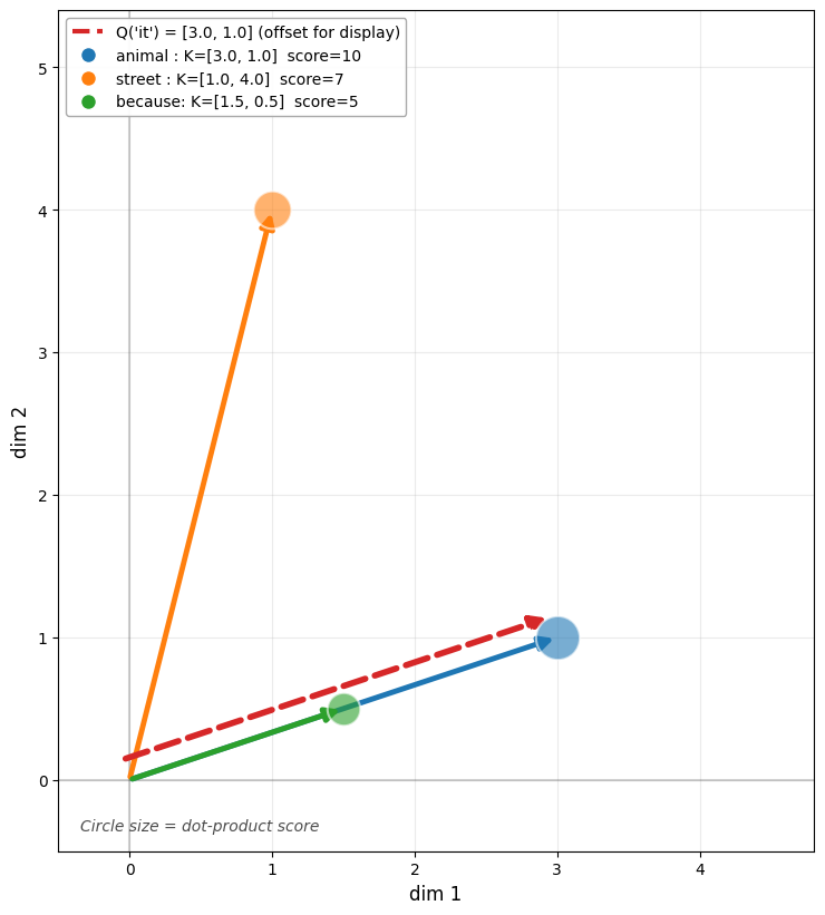
Step 1: Similarity in Q-K Space (Computing Scores)
import numpy as np
import matplotlib.pyplot as plt
from matplotlib.patches import FancyArrowPatch

def arrow(ax, start, end, color=None, lw=3, alpha=1.0, ls='-', z=3, ms=18):
    ax.add_patch(FancyArrowPatch(
        start, end,
        arrowstyle='-|>',
        mutation_scale=ms,
        linewidth=lw,
        linestyle=ls,
        color=color,
        alpha=alpha,
        zorder=z
    ))

def box(ax, x, y, text, fs=11, ha="left", va="top"):
    ax.text(
        x, y, text, fontsize=fs, ha=ha, va=va,
        transform=ax.transAxes,
        bbox=dict(boxstyle="round,pad=0.35", fc="white", ec="0.65", alpha=0.96)
    )

# Toy example aligned to your walkthrough
Q = np.array([3.0, 1.0])
K = {
    "animal":  np.array([3.0, 1.0]),
    "street":  np.array([1.0, 4.0]),
    "because": np.array([1.5, 0.5]),
}
names = list(K.keys())
scores = np.array([Q @ K[n] for n in names])

# Use matplotlib default color cycle (no hard-coded palette)
cycle = plt.rcParams['axes.prop_cycle'].by_key()['color']
colors = {n: cycle[i % len(cycle)] for i, n in enumerate(names)}
cQ = cycle[3 % len(cycle)]

fig, ax = plt.subplots(figsize=(7.5, 9))

# Offset Q slightly so it doesn't perfectly overlap K_animal
q_hat = Q / np.linalg.norm(Q)
perp = np.array([-q_hat[1], q_hat[0]])
eps = 0.15
q_start = eps * perp
q_end = q_start + Q
arrow(ax, (q_start[0], q_start[1]), (q_end[0], q_end[1]),
      color=cQ, lw=4, ls="--", z=5, ms=20)

# Keys with SAME thickness, but circle size proportional to score
smax = scores.max()
for i, n in enumerate(names):
    k = K[n]
    # Arrow points to the center of the circle at k[0], k[1]
    arrow(ax, (0, 0), (k[0], k[1]), color=colors[n], lw=3.5, z=4, ms=18)
    # Circle size proportional to score, doubled
    circle_size = 2 * (50 + 350 * (scores[i] / smax))
    ax.scatter([k[0]], [k[1]], s=circle_size, color=colors[n], alpha=0.6, zorder=6, edgecolors='white', linewidths=1.5)

# Color-coded legend with colored markers
from matplotlib.lines import Line2D
legend_elements = []

# Add Q line with note about offset
legend_elements.append(Line2D([0], [0], color=cQ, linestyle='--', lw=3,
                              label=f"Q('it') = {Q.tolist()} (offset for display)"))

# Add colored entries for each key
for i, n in enumerate(names):
    label_text = f"{n:7s}: K={K[n].tolist()}  score={scores[i]:.0f}"
    legend_elements.append(Line2D([0], [0], marker='o', color='w',
                                  markerfacecolor=colors[n], markersize=10,
                                  label=label_text))

ax.legend(handles=legend_elements, loc='upper left', fontsize=10,
          framealpha=0.95, edgecolor='0.65')

# Add note about circle sizes
ax.text(0.03, 0.02, "Circle size = dot-product score",
        fontsize=10, ha='left', va='bottom', transform=ax.transAxes,
        style='italic', alpha=0.7)

ax.axhline(0, color="k", alpha=0.18)
ax.axvline(0, color="k", alpha=0.18)
ax.grid(True, alpha=0.25)
ax.set_aspect("equal")
ax.set_xlabel("dim 1", fontsize=12)
ax.set_ylabel("dim 2", fontsize=12)
ax.set_xlim(-0.5, 4.8)
ax.set_ylim(-0.5, 5.4)

plt.tight_layout()
plt.show()
What this shows: The query “it” Q=[3, 1] (blue dashed arrow) compares against each key using the dot product. Notice that K_animal=[3, 1] perfectly aligns with Q (score=10), while K_street=[1, 4] points in a different direction (score=7). Circle size reflects the raw dot product scores—before any normalization.
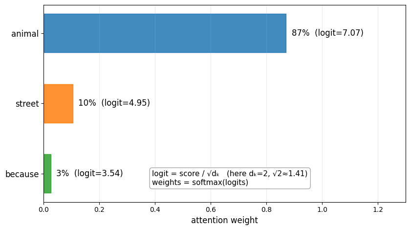
Steps 2-3: Scaling and Softmax (Scores → Weights)
import numpy as np
import matplotlib.pyplot as plt

def softmax(x):
    x = x - np.max(x)
    ex = np.exp(x)
    return ex / ex.sum()

def box(ax, x, y, text, fs=11, ha="left", va="top"):
    ax.text(
        x, y, text, fontsize=fs, ha=ha, va=va,
        transform=ax.transAxes,
        bbox=dict(boxstyle="round,pad=0.35", fc="white", ec="0.65", alpha=0.96)
    )

Q = np.array([3.0, 1.0])
K = {
    "animal":  np.array([3.0, 1.0]),
    "street":  np.array([1.0, 4.0]),
    "because": np.array([1.5, 0.5]),
}
names = list(K.keys())

d_k = Q.size
scores = np.array([Q @ K[n] for n in names])
logits = scores / np.sqrt(d_k)
w = softmax(logits)

cycle = plt.rcParams['axes.prop_cycle'].by_key()['color']
colors = {n: cycle[i % len(cycle)] for i, n in enumerate(names)}

fig, ax = plt.subplots(figsize=(8.5, 4.8))

y = np.arange(len(names))
bars = ax.barh(y, w, height=0.55)
for i, b in enumerate(bars):
    b.set_color(colors[names[i]])
    b.set_alpha(0.85)

ax.set_yticks(y, labels=names, fontsize=12)
ax.invert_yaxis()
ax.set_xlim(0, 1.3)
ax.set_xlabel("attention weight", fontsize=12)
ax.grid(True, axis="x", alpha=0.25)

for i, n in enumerate(names):
    ax.text(w[i] + 0.02, i, f"{w[i]*100:.0f}%  (logit={logits[i]:.2f})",
            va="center", fontsize=12)

box(ax, 0.3, 0.08, "logit = score / √dₖ   (here dₖ=2, √2≈1.41)\nweights = softmax(logits)",
    fs=11, va="bottom")

plt.tight_layout()
plt.show()
What this shows: We divide each score by √d_k=√2≈1.41 to get “logits”, then apply softmax to convert them into probabilities that sum to 1.0. The result: “animal” gets 87% of the attention (from score=10), “street” gets 10% (from score=7), and “because” gets 3% (from score=5). These are the attention weights.
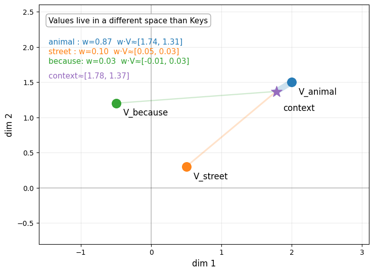
Step 4: Copy from Values (Weighted Sum in V-Space)
import numpy as np
import matplotlib.pyplot as plt

def softmax(x):
    x = x - np.max(x)
    ex = np.exp(x)
    return ex / ex.sum()

def box(ax, x, y, text, fs=11, ha="left", va="top"):
    ax.text(
        x, y, text, fontsize=fs, ha=ha, va=va,
        transform=ax.transAxes,
        bbox=dict(boxstyle="round,pad=0.35", fc="white", ec="0.65", alpha=0.96)
    )

Q = np.array([3.0, 1.0])
K = {
    "animal":  np.array([3.0, 1.0]),
    "street":  np.array([1.0, 4.0]),
    "because": np.array([1.5, 0.5]),
}
V = {
    "animal":  np.array([2.0, 1.5]),
    "street":  np.array([0.5, 0.3]),
    "because": np.array([-0.5, 1.2]),
}
names = list(K.keys())

d_k = Q.size
scores = np.array([Q @ K[n] for n in names])
logits = scores / np.sqrt(d_k)
w = softmax(logits)
context = sum(w[i] * V[names[i]] for i in range(len(names)))

cycle = plt.rcParams['axes.prop_cycle'].by_key()['color']
colors = {n: cycle[i % len(cycle)] for i, n in enumerate(names)}
cCTX = cycle[4 % len(cycle)]

fig, ax = plt.subplots(figsize=(7.5, 6.8))

# Plot value points
for i, n in enumerate(names):
    v = V[n]
    ax.scatter([v[0]], [v[1]], s=160, color=colors[n], alpha=0.95, zorder=4)
    ax.text(v[0] + 0.10, v[1] - 0.17, f"V_{n}", fontsize=12)

# Context point
ax.scatter([context[0]], [context[1]], s=260, color=cCTX, marker="*", zorder=6, alpha=0.95)
ax.text(context[0] + 0.10, context[1] - 0.27, "context", fontsize=12)

# Pull lines from context to values (thickness ~ weight)
for i, n in enumerate(names):
    v = V[n]
    lw = 1.5 + 7.0 * (w[i] / w.max())
    ax.plot([context[0], v[0]], [context[1], v[1]],
            linewidth=lw, alpha=0.22, color=colors[n], zorder=2)

# Draw the header box for the contribution summary
box(ax, 0.03, 0.95, "Values live in a different space than Keys", fs=11)

# Calculate starting Y position for the colored text lines
current_y = 0.86 # Adjusted to start below the header box

# Add color-coded contribution lines
for i, n in enumerate(names):
    text_line = f"{n:7s}: w={w[i]:.2f}  w·V≈[{(w[i]*V[n])[0]:.2f}, {(w[i]*V[n])[1]:.2f}]"
    ax.text(
        0.03, current_y, text_line, fontsize=11, ha="left", va="top",
        transform=ax.transAxes, color=colors[n]
    )
    current_y -= 0.04 # Move down for the next line

# Add some spacing before the context line
current_y -= 0.02

# Add context line with its specific color
ax.text(
    0.03, current_y,
    f"context≈[{context[0]:.2f}, {context[1]:.2f}]",
    fontsize=11, ha="left", va="top",
    transform=ax.transAxes, color=cCTX
)

ax.axhline(0, color="k", alpha=0.18)
ax.axvline(0, color="k", alpha=0.18)
ax.grid(True, alpha=0.25)
ax.set_aspect("equal")
ax.set_xlabel("dim 1", fontsize=12)
ax.set_ylabel("dim 2", fontsize=12)

pts = [context] + [V[n] for n in names]
xs = [p[0] for p in pts]
ys = [p[1] for p in pts]
ax.set_xlim(min(xs)-1.1, max(xs)+1.1)
ax.set_ylim(min(ys)-1.1, max(ys)+1.1)

plt.tight_layout()
plt.show()
What this shows: Values live in a different space than keys. Using the attention weights from Step 3, we compute a weighted average: context = 0.87×V_animal + 0.10×V_street + 0.03×V_because ≈ [1.78, 1.37]. The thick line to V_animal shows it dominates the contribution. This final context vector becomes the new representation for “it”—enriched with semantic content from “animal”.
Key Insight: Attention is a weighted average in value space, where the weights come from measuring similarity in query-key space. This is fundamentally different from a traditional database lookup:
Traditional database: Query finds exact key matches → retrieves paired value (e.g., user_id=123 → user data)
This is why we need separate Q, K, V projections: K and V are different learned transformations of the same input. Keys determine how much to attend (semantic matching via geometric alignment), while Values determine what information to extract (the content to mix into the output). K[“river”] might encode “geographic term, noun, concrete” (optimized for matching), while V[“river”] encodes “flowing water, nature, geography” (semantic content to contribute).