L02 - Embeddings & Positional Encoding: Giving Numbers Meaning

How words become vectors in space, and how we tell time without a clock

In L01 - Tokenization, we turned text into IDs. But to a neural network, ID 464 and ID 465 are just arbitrary numbers. There is no inherent relationship between them.

In this post, we solve two problems:

Meaning: How do we represent words so that “King” is mathematically closer to “Queen” than it is to “Toaster”?
Order: Since the attention-based model we’ll build in the next lesson processes all tokens at once, how do we tell it that “The dog bit the man” is different from “The man bit the dog”?

By the end of this post, you’ll understand:

The intuition of Embedding Spaces.
How to implement a lookup table from scratch.
The beautiful math behind Sinusoidal Positional Encodings.

import os
import logging
import warnings

logging.getLogger("matplotlib.font_manager").setLevel(logging.ERROR)
warnings.filterwarnings("ignore", message="Matplotlib is building the font cache*")

import matplotlib
import numpy as np

import matplotlib.pyplot as plt

plt.rcParams['figure.facecolor'] = 'white'
plt.rcParams['axes.facecolor'] = 'white'

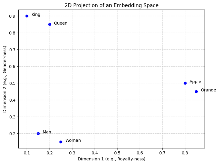
Part 1: The Embedding Space¶

Imagine every word is a point in a high-dimensional room. Words with similar meanings are “clumped” together. This is an Embedding Space.

An Embedding Layer is simply a big lookup table. If our vocabulary size is 10,000 and we want each word to be represented by a vector of 512 numbers, our table is a $10,000 \times 512$ matrix.

The Lookup Operation¶

When the model sees ID 5, it doesn’t do math on the number 5. It simply grabs the 5th row of the embedding matrix.

# Simplified 2D Embedding Visualization
words = ["King", "Queen", "Man", "Woman", "Apple", "Orange"]
# Arbitrary coordinates to show relationships
coords = np.array([
    [0.1, 0.9], [0.2, 0.85], # Royalty
    [0.15, 0.2], [0.25, 0.15], # People
    [0.8, 0.5], [0.85, 0.45]  # Fruit
])

plt.figure(figsize=(8, 6))
plt.scatter(coords[:, 0], coords[:, 1], color='blue')

for i, word in enumerate(words):
    plt.annotate(word, (coords[i, 0]+0.02, coords[i, 1]))

plt.title("2D Projection of an Embedding Space")
plt.xlabel("Dimension 1 (e.g., Royalty-ness)")
plt.ylabel("Dimension 2 (e.g., Gender-ness)")
plt.grid(True, linestyle='--', alpha=0.6)
plt.show()

Part 2: The Problem of Order¶

Standard Neural Networks (like the MLPs we built in the Neural Networks from Scratch series) process data in a specific order. The attention mechanism we’ll introduce next is parallel. It looks at every word in a sentence at the exact same time.

Without help, the attention-based model sees the sentence “The dog bit the man” as a bag of words. It has no idea which word came first.

We fix this by adding Positional Encodings.

Part 3: Positional Encoding (The Sine/Cosine Trick)¶

This is often the most confusing part of the Transformer architecture, so let’s derive it from scratch.

The Problem: Why not just count?¶

If we want to represent the order of words, the simplest idea is to just assign an integer to each position:

“The” $\rightarrow$ 1
“Dog” $\rightarrow$ 2
“Bit” $\rightarrow$ 3

Why this fails:

Exploding Values: For a long document, the 5,000th word would have the value 5000. Neural networks hate large, unbounded numbers; they cause gradients to explode and training to become unstable.
Inconsistent Steps (if normalized): You might try dividing by the total length (e.g., $0.0, 0.5, 1.0$ for a 3-word sentence). But then the “time distance” between words changes depending on the sentence length. We need a method where the step size is bounded and consistent.

The Intuition: The “Binary Clock”¶

So, how do we represent numbers that get bigger and bigger without using huge values? We use patterns. Think of how binary numbers work.

Let’s start with a simple 3-bit binary counter to see the pattern clearly:

Position	Bit 2 (Slow)	Bit 1 (Medium)	Bit 0 (Fast)	Binary
0	0	0	0	`000`
1	0	0	1	`001`
2	0	1	0	`010`
3	0	1	1	`011`
4	1	0	0	`100`
5	1	0	1	`101`
6	1	1	0	`110`
7	1	1	1	`111`

Notice the pattern?

Bit 0 (Fast) alternates every single step: $0, 1, 0, 1, 0, 1, 0, 1$ (High Frequency).
Bit 1 (Medium) alternates every two steps: $0, 0, 1, 1, 0, 0, 1, 1$ (Lower Frequency).
Bit 2 (Slow) alternates every four steps: $0, 0, 0, 0, 1, 1, 1, 1$ (Lowest Frequency).

Each column oscillates at a different frequency. Together, they create a unique combination for every row, using only 0s and 1s.

From Binary to Continuous (The Spectrum)¶

Transformers adapt this binary idea using continuous waves (Sine and Cosine). But instead of just “fast” and “slow,” we have a smooth spectrum of frequencies across the embedding dimensions.

Dimension 0 (The Seconds Hand): The wave wiggles extremely fast. A small change in position causes a huge change in value. This gives the model precision (distinguishing word #5 from #6).
Dimension 100...: The frequency gradually slows down.
Dimension 512 (The Hour Hand): The wave wiggles extremely slowly. This gives the model long-term context (distinguishing word #5 from #5000).

The Formula¶

For a position $pos$ and dimension index $j$ :

Even dimensions ( $2i$ ) use Sine.
Odd dimensions ( $2i+1$ ) use Cosine.

PE_{(pos, 2i)} = \sin\left(\frac{pos}{10000^{2i/d_{model}}}\right)

(1)

PE_{(pos, 2i+1)} = \cos\left(\frac{pos}{10000^{2i/d_{model}}}\right)

(2)

Don’t let the 10000^... term scare you. It is just a “wavelength knob.” Let’s plug in some real numbers to see it in action.

Example: Plugging in the Numbers

Imagine we have a model with $d_{model} = 512$ . This means we have 256 pairs of Sine/Cosine waves.

Case 1: The “Fast” Pair (Dimensions 0 & 1) We are at the start of the vector ( $i=0$ ).

\text{Denominator} = 10000^0 = 1

(3)

Dim 0: $\sin(pos/1)$ $\rightarrow$ Wiggles every ~6 words.
Dim 1: $\cos(pos/1)$ $\rightarrow$ Same speed, just shifted.

This pair acts like the “Seconds Hand” (High Precision).

Case 2: The “Slow” Pair (Dimensions 510 & 511) We are at the end of the vector ( $i=255$ ).

\text{Denominator} = 10000^{510/512} \approx 10000

(4)

Dim 510: $\sin(pos/10000)$
Dim 511: $\cos(pos/10000)$

This pair acts like the “Hour Hand” (Long-term Context). It takes ~62,800 words to complete one cycle!

Wait, aren’t all embedding dimensions supposed to be equal?

In a standard embedding (like word2vec), yes—Dimension 0 and Dimension 511 are just arbitrary “buckets” for numbers. They start equal.

Positional Encoding changes this. By adding these fixed waves, we are strictly enforcing a hierarchy onto the dimensions:

Low Dimensions (0-63) become the “High Frequency / Precision” channels. They change rapidly with position, helping the model distinguish adjacent words.
Middle Dimensions (64-255) capture medium-range patterns, useful for understanding phrases and clauses.
High Dimensions (256-511) become the “Low Frequency / Context” channels, encoding long-range dependencies across sentences or paragraphs.

The model is smart enough to adapt to this structure. During training, it learns to store semantic information in a way that complements these positional frequencies. Think of it like this: the embedding provides the “what” (word meaning), while the positional encoding provides the “when” (word position), and the model learns to separate and use both signals effectively.

Example: The word “bank” might have similar embeddings at positions 5 and 50, but the positional encoding ensures the model knows these are different tokens in the sequence. The high-frequency dimensions will differ significantly, while low-frequency dimensions might be similar for nearby positions.

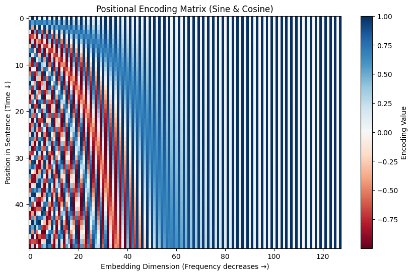
Visualization¶

Let’s generate the matrix. In the plot below:

X-axis: The Embedding Dimensions (0 to 128).
Y-axis: The Position in the sentence (0 to 50).
Color: The value (Blue is negative, Red is positive).

Notice the “barber pole” pattern? That is the frequencies getting slower as you move to the right (higher dimensions).

def get_positional_encoding(max_seq_len, d_model):
    pe = np.zeros((max_seq_len, d_model))
    for pos in range(max_seq_len):
        for i in range(0, d_model, 2):
            div_term = np.exp(i * -(np.log(10000.0) / d_model))
            pe[pos, i] = np.sin(pos * div_term)
            pe[pos, i + 1] = np.cos(pos * div_term)
    return pe

d_model = 128
max_len = 50
pe = get_positional_encoding(max_len, d_model)

plt.figure(figsize=(10, 6))
plt.imshow(pe, cmap='RdBu', aspect='auto')
plt.colorbar(label='Encoding Value')
plt.title("Positional Encoding Matrix (Sine & Cosine)")
plt.xlabel("Embedding Dimension (Frequency decreases →)")
plt.ylabel("Position in Sentence (Time ↓)")
plt.show()

Alternative Approach: Learned Positional Embeddings

While sinusoidal positional encoding is elegant and works well, many models (like GPT-2 and BERT) use learned positional embeddings instead. Rather than using a fixed mathematical formula, these models treat positional encodings as trainable parameters—just like word embeddings.

Advantages:

The model can learn the optimal positional representation for the specific task
Simpler implementation (just another embedding table)
Often works slightly better in practice

Disadvantages:

Fixed maximum sequence length (sinusoidal can theoretically extrapolate to longer sequences)
Requires learning during training (more parameters)

In code, this looks like:

self.pos_embedding = nn.Embedding(max_seq_len, d_model)

Both approaches are valid, and the choice often comes down to implementation preference and specific use case requirements.

Part 4: Putting it Together¶

The final input to our model is:

\text{Input} = \text{Embedding}(w) + \text{PositionalEncoding}(pos)

(5)

Now, the vector for “dog” at position 2 is slightly different from the vector for “dog” at position 5. The “meaning” is the same, but the “stamp” of its location is unique.

# Pseudo-code for the input pipeline
word_ids = [464, 2068, 7586] # "The quick brown"
embeddings = embedding_layer(word_ids) # Shape: [3, 512]
positions = positional_encoding_layer(range(len(word_ids))) # Shape: [3, 512]

final_input = embeddings + positions

Concrete Example: What the Numbers Look Like¶

Let’s see what these vectors actually contain (showing just the first 8 dimensions out of 512):

# Token: "The" (position 0)
embedding_The = [ 0.21,  0.15, -0.33,  0.08, -0.12,  0.19,  0.05, -0.28, ...]  # Learned
pos_encoding_0 = [ 0.00,  1.00,  0.00,  1.00,  0.00,  1.00,  0.00,  1.00, ...]  # Fixed (sin/cos)
final_input_0  = [ 0.21,  1.15, -0.33,  1.08, -0.12,  1.19,  0.05,  0.72, ...]  # Sum

# Token: "quick" (position 1)
embedding_quick = [-0.18,  0.42,  0.11, -0.25,  0.37, -0.14,  0.22,  0.09, ...]  # Learned
pos_encoding_1  = [ 0.84,  0.54,  0.10,  0.99,  0.01,  1.00,  0.00,  1.00, ...]  # Fixed (sin/cos)
final_input_1   = [ 0.66,  0.96,  0.21,  0.74,  0.38,  0.86,  0.22,  1.09, ...]  # Sum

# Token: "brown" (position 2)
embedding_brown = [ 0.09, -0.31,  0.44,  0.17, -0.08,  0.26, -0.13,  0.35, ...]  # Learned
pos_encoding_2  = [ 0.91, -0.42,  0.20,  0.98,  0.02,  1.00,  0.00,  1.00, ...]  # Fixed (sin/cos)
final_input_2   = [ 1.00, -0.73,  0.64,  1.15, -0.06,  1.26, -0.13,  1.35, ...]  # Sum

Key observations:

Embeddings have learned values (positive and negative) that capture word meaning
Positional encodings follow the sin/cos pattern (notice the periodic structure)
Final input is simply the element-wise sum of the two
Same word at different positions gets different final vectors (different PE added)

Summary¶

Embeddings map discrete IDs to continuous vectors where distance equals similarity.
Positional Encodings inject a sense of order into a model that otherwise sees everything at once.
Addition: We simply add these two vectors together. The model learns to separate the “meaning” signal from the “position” signal during training.

Embeddings at Scale Book:

Next Up: L03 – The Attention Mechanism. This is the “Aha!” moment of the entire series. We will build the logic that allows the model to decide which words in a sentence are most relevant to each other.