This chapter is being updated to reflect the VAST Data Platform Vector DB architecture. Sections on sharding, replication, and distribution patterns will be revised to cover VAST-specific approaches. The foundational concepts (indexing algorithms, SLA design, benchmarking) remain applicable.
NoteChapter Overview
This chapter covers vector database architecture principles, indexing strategies for 256+ trillion rows, distributed systems considerations, performance benchmarking and SLA design, and data locality patterns for global-scale embedding deployments.
3.1 Vector Database Architecture Principles
Traditional databases were designed for exact matches: “Find customer with ID=12345” or “Return all orders where status=‘shipped’”. Vector databases serve a fundamentally different purpose: finding semantic similarity in high-dimensional space. This section explores the architectural principles that make trillion-row vector search possible.
3.1.1 Why Traditional Databases Fail for Embeddings
The scale mismatch becomes clear with a simple calculation:
# Traditional database querydef find_customer(database, customer_id):"""O(log N) with B-tree index"""return database.index['customer_id'].lookup(customer_id)# 256 trillion rows: ~48 comparisons# Naive embedding searchdef find_similar_naive(query_embedding, all_embeddings):"""O(N * D) where N=rows, D=dimensions""" similarities = []for embedding in all_embeddings: # 256 trillion iterations similarity = cosine_similarity(query_embedding, embedding) # 768 multiplications similarities.append(similarity)return top_k(similarities, k=10)# Cost calculation:# 256 trillion rows × 768 dimensions = 196 quadrillion operations# At 1 billion ops/second: 6 years per query
Traditional databases optimize for exact lookups and range scans. Vector databases optimize for approximate nearest neighbor (ANN) search in high-dimensional space. These are fundamentally different problems requiring different architectures.
3.1.2 The Core Architectural Principles
Principle 1: Approximate is Sufficient
Unlike financial transactions where precision is mandatory, embedding similarity is inherently approximate. Whether an item is the 47th or 48th most similar out of 256 trillion doesn’t matter—both are highly relevant.
This insight unlocks massive performance gains:
Aspect
Traditional DB
Vector DB
Correctness
100% exact
95-99% approximate
Performance
O(log N) with index
O(log N) even without perfect accuracy
Use Case
Exact match, transactions
Semantic similarity, recommendations
The key insight: trading a small amount of accuracy for massive speed gains. Finding the top-10 most similar items from 256T vectors via exact search is infeasible—approximate nearest neighbor (ANN) algorithms achieve 95%+ recall in milliseconds.
Principle 2: Geometry Matters More Than Algebra
Vector databases exploit geometric structure rather than brute-force computation. Similar embeddings cluster together in space, and similarity metrics like cosine and Euclidean distance have properties that enable clever indexing shortcuts. For a detailed comparison of these metrics and when to use each, see Chapter 2.
Principle 3: Index Structure is Everything
You don’t need to compare against all vectors—the right index structure lets you navigate efficiently. The choice determines performance, accuracy, and scalability:
Index
Build Time
Query Time
Memory
Accuracy
Max Scale
Use Case
Flat
O(N)
O(N×D)
O(N×D)
100%
~1M
Ground truth
IVF
O(N×k)
O((N/k)×D×n_probe)
O(N×D+k×D)
80-95%
~1B
Balanced
HNSW
O(N×log(N)×M)
O(log(N)×M)
O(N×(D+M))
95-99%
100B+
Production (best tradeoff)
LSH
O(N×L)
O(L×bucket)
O(N×L)
70-90%
Trillion+
Ultra-massive scale
PQ
O(N×iter)
O(N) compressed
O(N×code)
85-95%
10B+
Memory-constrained
HNSW is the gold standard for high-performance production systems due to its best accuracy/speed tradeoff at scale.
NoteVAST Data Platform Approach
This section will cover VAST Data Platform’s approach to data distribution and storage architecture, which differs from traditional sharding patterns. VAST’s unified storage architecture eliminates many of the manual sharding decisions required by other vector databases.
ImportantArchitecture First, Scaling Later
The most expensive mistake: starting with single-node architecture and retrofitting for scale. Design for distribution from day one, even if you start with one machine. The patterns are the same, only the scale changes.
3.2 Indexing Strategies at Scale
Scaling to trillions of embeddings requires sophisticated indexing strategies that balance accuracy, speed, memory, and build time. This section explores battle-tested approaches.
3.2.1 The Indexing Challenge at Scale
Before diving into solutions, let’s quantify what 1 trillion 768-dimensional vectors actually means:
Storage: Each vector is 768 floats × 4 bytes = 3KB. One trillion vectors = ~2.8 PB raw, plus ~50% overhead for HNSW graph structure.
Memory cost: If you wanted everything in RAM, you’d need thousands of high-memory machines at tens of millions per month.
Build time: HNSW takes ~100μs per vector insertion. Single-threaded, that’s years. Even with massive parallelism, it’s a significant operation.
Query budget: Users expect results in under 100ms. After network and processing overhead, the index search itself gets maybe 50ms—no room for brute force.
Show the math
# Scale parametersnum_vectors =1_000_000_000_000# 1 trillionembedding_dim =768bytes_per_float =4# Storage calculationraw_petabytes = (num_vectors * embedding_dim * bytes_per_float) / (1024**5)with_index_pb = raw_petabytes *1.5# HNSW adds ~50% overhead# Cost if all in RAM (AWS r6i.32xlarge: 1TB RAM, $8.064/hour)machines_1tb =int(with_index_pb *1024)monthly_cost = machines_1tb *8.064*24*30# Build time (~100μs per vector for HNSW)build_seconds = (num_vectors *100) /1_000_000build_years = build_seconds / (60*60*24*365)parallel_hours = (build_seconds /10_000) / (60*60) # With 10K machinesprint(f"Storage: {with_index_pb:,.0f} PB (embeddings + HNSW index)")print(f"Machines: {machines_1tb:,} × 1TB RAM instances")print(f"Cost: ${monthly_cost/1e6:,.0f}M/month if all in RAM")print(f"Build time: {build_years:,.0f} years single-machine, {parallel_hours:.0f} hours with 10K machines")print(f"Query: Must return results in <50ms (no room for brute force)")
Storage:    4 PB (embeddings + HNSW index)
Machines:   4,190 × 1TB RAM instances
Cost:       $24M/month if all in RAM
Build time: 3 years single-machine, 3 hours with 10K machines
Query:      Must return results in <50ms (no room for brute force)
Clearly, naïve approaches won’t work. We need sophisticated indexing strategies.
3.2.2 Strategy 1: Hierarchical Navigable Small World (HNSW)
HNSW is the gold standard for high-recall, low-latency vector search. Understanding how it works is essential for trillion-scale deployments.
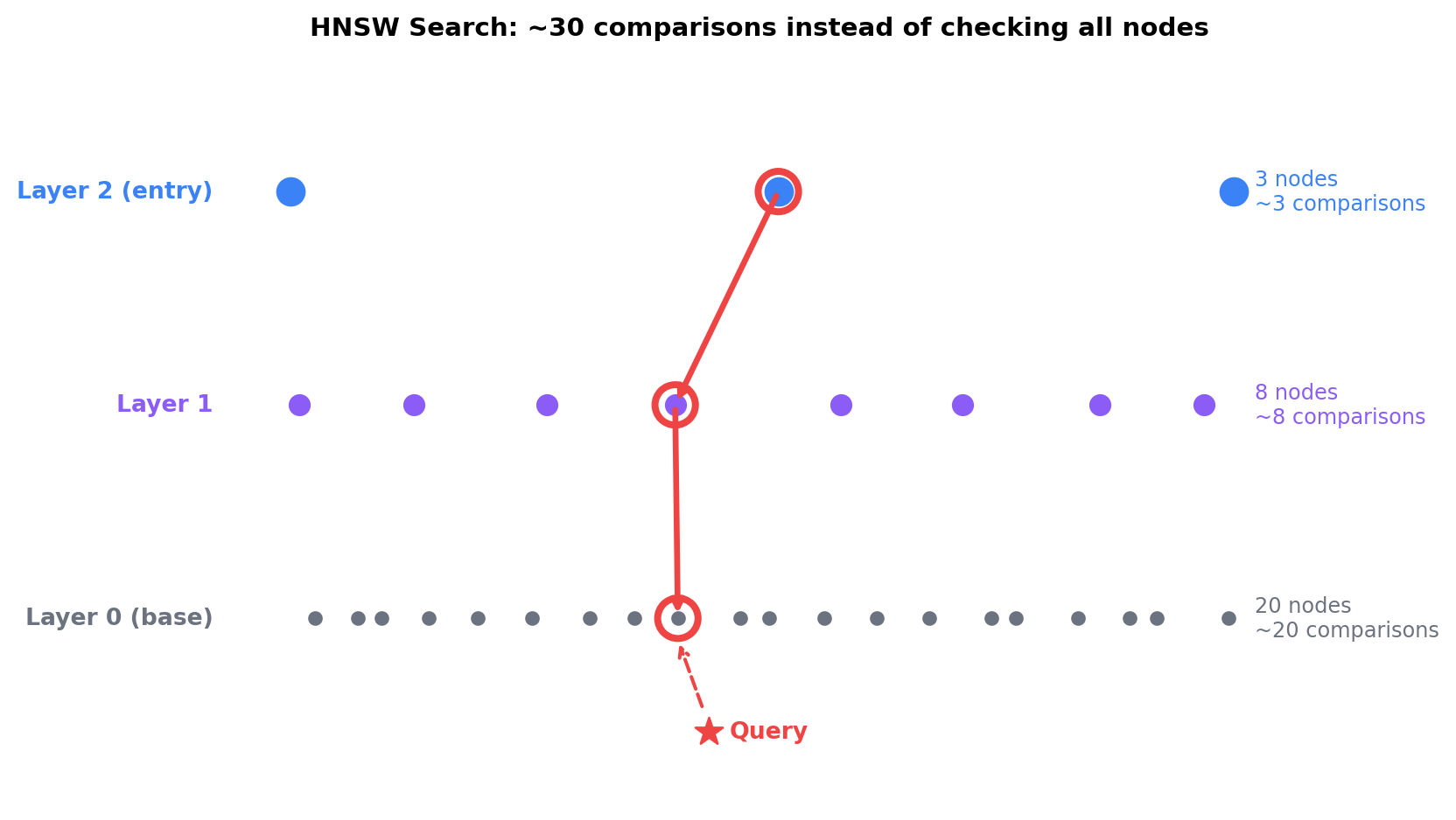
Core Concept: HNSW builds a multi-layer graph where each vector is randomly assigned to a level (higher levels are exponentially rarer). Within each layer, vectors connect to their nearest neighbors. The key insight:
Upper layers: Few nodes, spread far apart → each hop covers large distances
Bottom layer: All nodes, densely packed → each hop is fine-grained
Search: Enter at top, greedily hop toward query, descend when stuck
Figure 3.1: HNSW navigation: enter at sparse top layer, greedily hop to neighbors closest to query, descend when you can’t improve. With 1T vectors in ~15 layers, this turns O(N) brute force into O(log N) traversal.
Tuning HNSW Parameters
Parameter
What it controls
Small (1M)
Medium (100M)
Large (1B+)
M
Connections per node
16
32
48-64
ef_construction
Build quality (candidates considered)
100
200
400
ef_search
Query quality vs speed
50
100
200
Higher M and ef values improve recall but increase memory and latency. At 1B vectors with M=48, expect ~6 layers and ~300 comparisons per query—orders of magnitude faster than brute force.
3.2.3 Strategy 2: IVF (Inverted File Index) with Product Quantization
While HNSW is excellent for recall and latency, IVF-PQ excels at massive scale with memory constraints.
Core Concept: IVF-PQ combines two techniques:
IVF (Inverted File): Partition vectors into clusters using k-means. At query time, only search the nearest clusters instead of all vectors.
Product Quantization (PQ): Split each vector into subvectors and quantize each independently. A 768-dim vector becomes ~96 bytes instead of 3KB—32x compression.
Figure 3.2: IVF-PQ: (Left) IVF partitions space into clusters—query searches only nearby cells (green), skipping distant ones (gray). (Right) PQ compresses each vector by splitting into subvectors and storing cluster IDs instead of floats.
Tuning IVF-PQ Parameters
Parameter
What it controls
Small (10M)
Medium (1B)
Large (100B+)
nlist
Number of clusters
1,024
16,384
65,536
nprobe
Clusters to search
8
64
128
M (PQ)
Subquantizers
16
48
96
Higher nprobe improves recall but increases latency. At 100B vectors with 96 subquantizers, expect 32x compression (286 TB → 9 TB) with 85-90% recall.
Hybrid IVF-HNSW: Best of both—IVF for coarse search, HNSW within partitions
3.2.4 Strategy 3: Data Distribution at Scale
At trillion scale, efficient data distribution is essential for performance and availability.
NoteVAST Data Platform Approach
This section will cover VAST Data Platform’s approach to data distribution, which provides automatic scaling and data placement without manual sharding configuration. VAST’s architecture handles data distribution transparently, eliminating the complexity of traditional sharding strategies.
3.3 Distributed Systems Considerations
Vector databases at trillion-scale are distributed systems, inheriting all the challenges of distributed computing: consistency, availability, partition tolerance, and coordination.
3.3.1 The CAP Theorem for Vector Databases
Vector databases choose AP (Availability + Partition Tolerance) over strong consistency. This is the right tradeoff because embeddings are inherently approximate—if one replica has slightly outdated embeddings, query results are still useful.
Consistency requirements by operation:
Writes/Inserts: Eventual consistency. Write to primary, async replicate. New embedding visible within 5 seconds.
Updates/Deletions: Eventual consistency with tombstones. Deleted items filtered at query time.
Reads/Queries: Read-your-writes for same session (via session affinity). May see stale data from other users—acceptable.
Metadata filters: Strong consistency required. Security filters (user access) must be immediate.
Availability techniques: 3x replication, read from any replica, automatic failover, circuit breakers. Target: 99.99%.
Partition tolerance: Gracefully degrade by serving cached results, partial results from available shards, or falling back to multi-region replicas.
3.3.2 Replication and Data Protection
Data replication ensures availability and durability at scale.
NoteVAST Data Platform Approach
This section will cover VAST Data Platform’s built-in data protection and failure recovery mechanisms, including:
Data Protection: VAST’s approach to erasure coding and data redundancy
Automatic Failover: How VAST handles node and disk failures transparently
Disaster Recovery: Multi-site replication and recovery capabilities
Self-Healing: Automatic detection and recovery from failures
VAST provides enterprise-grade reliability without requiring manual configuration of replication, sharding, or failover logic.
3.3.3 Coordination and Cluster Management
Distributed vector databases require coordination for metadata management and cluster operations.
NoteVAST Data Platform Approach
This section will cover how VAST Data Platform handles cluster coordination and management. VAST’s architecture simplifies operational complexity by providing integrated cluster management without external coordination services like ZooKeeper or etcd.
3.4 Performance Benchmarking and SLA Design
Production vector databases require rigorous SLA design and continuous performance monitoring. This section covers benchmarking methodologies and SLA patterns.
SLA (Service Level Agreement): Contract with consequences (e.g., “p99 < 100ms or 10% credit”)
3.4.2 Benchmarking Methodology
Key benchmark dimensions for vector databases:
Category
Metrics
Variables
Index Build
Build time, throughput (vec/sec), peak memory, CPU
Dataset size, dimensions, index params (M, ef)
Query
p50/p95/p99 latency, QPS, recall@10/100
K, ef_search, query distribution, concurrency
Updates
Insert latency/throughput, recall drift
Insert rate, update fraction
Scalability
Latency/memory vs size
Test at 1M, 10M, 100M, 1B, 10B vectors
Standard benchmark datasets include SIFT-1M (1M vectors, 128 dims), Deep1B (1B vectors, 96 dims), and LAION-5B (5B vectors, 768 dims). However, production data provides the most accurate benchmarks since query distributions differ from academic datasets.
3.4.3 Load Testing and Capacity Planning
Essential load test scenarios for vector databases:
Steady State: Maintain target QPS (e.g., 100K) for 1 hour. Verify p99 <100ms, no errors, stable resource usage.
Ramp Up: Gradually increase 0→200K QPS over 30 minutes to find breaking point and verify graceful degradation.
Spike: Sudden burst (50K→500K QPS for 5 minutes) to test autoscaling—system should scale within 2 minutes.
Sustained Peak: 150K QPS for 8 hours to detect memory leaks and resource exhaustion.
Thundering Herd: 1M simultaneous requests to test queue depth control and load shedding.
Geographic: Multi-region simultaneous load to verify routing and cross-region failover.
For capacity planning, assume ~10K QPS per shard and maintain 2x headroom for spikes. With 50% YoY growth, plan 3 years ahead: 100K QPS today requires 20 shards with headroom, growing to 68 shards by year 3.
3.5 Data Locality and Global Distribution
For trillion-row systems serving global users, data locality and geographic distribution are critical for latency and compliance.
NoteVAST Data Platform Approach
This section will cover VAST Data Platform’s approach to global data distribution, including:
Geographic Distribution: How VAST handles multi-region deployments and data placement
Data Residency: VAST’s capabilities for GDPR, CCPA, and regional compliance requirements
Latency Optimization: Built-in mechanisms for minimizing query latency across regions
Global Namespace: VAST’s unified approach to accessing data across locations
VAST provides enterprise-grade global distribution without requiring manual configuration of replication patterns or regional sharding.
3.6 Key Takeaways
Vector databases are fundamentally different from traditional databases—optimized for approximate nearest neighbor search in high-dimensional space rather than exact matches, making approximate results and geometric reasoning core architectural principles
HNSW is the gold standard for high-recall, low-latency search at billion to trillion scale, achieving O(log N) query complexity through hierarchical graph navigation, with typical configurations (M=32-64, ef_construction=200-400) delivering 95-99% recall at <100ms p99
IVF-PQ provides extreme memory efficiency with 20-100x compression through coarse quantization and product quantization, making it the best choice for memory-constrained trillion-scale deployments despite slightly lower recall (85-95%)
Data distribution is essential at trillion-scale—modern platforms like VAST Data Platform handle distribution automatically, while traditional approaches require manual sharding with configurations of 100M-1B vectors per partition
Vector databases choose AP over C in the CAP theorem, prioritizing availability and partition tolerance with eventual consistency for embeddings (acceptable due to inherent approximation) while maintaining strong consistency for critical metadata like access controls
SLA design requires percentile-based latency targets (p99 <100ms is typical), recall guarantees (>95% recall@10), and availability targets (99.99%), measured continuously with public dashboards and automated alerting on violations
Global distribution requires geographic strategies—full replication for lowest latency (5x cost), regional sharding for data sovereignty (lower cost), tiered distribution for balanced cost/latency (60-80% savings), or edge caching for popular queries (85-95% hit rates)
3.7 Looking Ahead
Part II begins with Chapter 4, exploring text embeddings—the most common type you’ll encounter. You’ll learn to create embeddings for words, sentences, and documents, with an optional “Advanced” section explaining how models like Word2Vec, BERT, and Sentence Transformers work under the hood. Subsequent chapters cover image, multi-modal, graph, time-series, and code embeddings.
3.8 Further Reading
Malkov, Y. A., & Yashunin, D. A. (2018). “Efficient and robust approximate nearest neighbor search using Hierarchical Navigable Small World graphs.” IEEE Transactions on Pattern Analysis and Machine Intelligence
Jégou, H., Douze, M., & Schmid, C. (2011). “Product Quantization for Nearest Neighbor Search.” IEEE Transactions on Pattern Analysis and Machine Intelligence
Johnson, J., Douze, M., & Jégou, H. (2019). “Billion-scale similarity search with GPUs.” IEEE Transactions on Big Data
Aumüller, M., Bernhardsson, E., & Faithfull, A. (2020). “ANN-Benchmarks: A Benchmarking Tool for Approximate Nearest Neighbor Algorithms.” Information Systems
Brewer, E. A. (2012). “CAP twelve years later: How the ‘rules’ have changed.” Computer
Gormley, C., & Tong, Z. (2015). Elasticsearch: The Definitive Guide. O’Reilly Media
Kleppmann, M. (2017). Designing Data-Intensive Applications. O’Reilly Media
Beyer, B., et al. (2016). Site Reliability Engineering: How Google Runs Production Systems. O’Reilly Media