1 The Embedding Revolution
NoteChapter Overview
This chapter begins with the fundamentals of what embeddings are and their key properties, then explores why they have become a competitive advantage for organizations and how they transform everything from search to reasoning. We examine the technical evolution, establish frameworks for understanding embedding moats, and provide practical ROI calculation methods.
1.1 What Are Embeddings?
Before we explore why embeddings are revolutionizing industries, let’s establish what embeddings actually are and why they represent such a fundamental shift in how we represent and process information.
1.1.1 The Core Concept
At their most basic, embeddings are numerical vectors that represent objects in a continuous multi-dimensional space. Think of them as coordinates on a map, but instead of just two dimensions (latitude and longitude), embeddings typically use hundreds or thousands of dimensions to capture the nuances of complex objects like words, images, products, or users.
TipTerminology: Embeddings = Vectors
The terms “embedding” and “vector” are used interchangeably throughout this book and in the industry. An embedding is a vector—a list of numbers like [0.2, -0.5, 0.8, ...]. We say “embedding” when emphasizing the semantic meaning captured by the numbers, and “vector” when emphasizing the mathematical operations we perform on them.
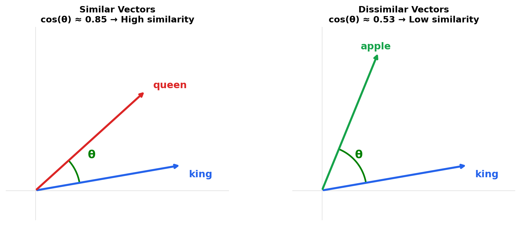
Here’s the key insight: in an embedding space, similarity in meaning corresponds to proximity in geometric space. Objects that are conceptually related end up close to each other, while unrelated objects are far apart.
"""
Word Embeddings Similarity Example

Demonstrates the core concept of embeddings: numerical vectors that represent
objects in a continuous multi-dimensional space, where similarity in meaning
corresponds to proximity in geometric space.

A simple 3-dimensional embedding space for illustration

Why 3 dimensions? This is deliberately simplified for visualization and pedagogy.
Real embeddings typically use 300-1024 dimensions, but 3D allows us to:
- Visualize the concept geometrically (x, y, z axes)
- Understand the math without getting lost in high-dimensional space
- Demonstrate the core principle: semantic similarity = geometric proximity

How were these values chosen? They're hand-crafted to demonstrate key relationships:
- Dimension 0 (~0.9 or ~0.5): Represents "royalty" vs "common"
- Dimension 1 (~0.8 or ~0.2): Represents "human" vs "other"
- Dimension 2 (~0.1 or ~0.9): Represents "male" vs "female"
(In real embeddings, dimensions aren't this interpretable—they're learned automatically)
"""
from scipy.spatial.distance import cosine

word_embeddings = {
    "king":  [0.9, 0.8, 0.1],  # Royal + human + male
    "queen": [0.9, 0.8, 0.9],  # Royal + human + female
    "man":   [0.5, 0.8, 0.1],  # Common + human + male
    "woman": [0.5, 0.8, 0.9],  # Common + human + female
    "apple": [0.1, 0.3, 0.5],  # Not royal, not human, neutral
}

def similarity(word1, word2):
    """Calculate cosine similarity between two word embeddings (1 = identical, 0 = unrelated)."""
    return 1 - cosine(word_embeddings[word1], word_embeddings[word2])


# Demonstrate that related words have similar embeddings
print(f"king vs queen: {similarity('king', 'queen'):.3f}")  # High (~0.85) - both royalty
print(f"man vs woman: {similarity('man', 'woman'):.3f}")    # High (~0.80) - both human
print(f"king vs apple: {similarity('king', 'apple'):.3f}")  # Low  (~0.53) - unrelated concepts
king vs queen: 0.848
man vs woman: 0.792
king vs apple: 0.532In this toy example, ‘king’ and ‘queen’ have similar embeddings because they’re related concepts (both royalty). ‘King’ and ‘apple’ are dissimilar because they’re unrelated.
TipUnderstanding Cosine Similarity
Cosine similarity measures how similar two vectors are by calculating the cosine of the angle between them—it asks “are these vectors pointing in the same direction?” regardless of their lengths.
Values range from 1.0 (identical direction) to -1.0 (opposite direction), with 0 meaning unrelated. Crucially, cosine similarity ignores magnitude—[1, 2, 3] and [2, 4, 6] have similarity of 1.0 because they point in the same direction.
Warning
Similarity vs Distance: Some functions return cosine distance (1 - similarity) where lower = more similar. For example, scipy.spatial.distance.cosine() returns distance, while sklearn.metrics.pairwise.cosine_similarity() returns similarity. Always check which convention a function uses!
For the mathematical formula, worked examples, and comparison with other metrics (Euclidean, dot product, Manhattan, etc.), see Chapter 2.
1.1.2 From Discrete to Continuous: Why Embeddings Matter
Traditional computer systems represent objects discretely. Consider how we might represent words:
One-hot encoding (traditional approach):
# Each word is a unique, independent identifier
vocabulary = ['cat', 'dog', 'kitten', 'puppy', 'car']

one_hot = {
    'cat':    [1, 0, 0, 0, 0],
    'dog':    [0, 1, 0, 0, 0],
    'kitten': [0, 0, 1, 0, 0],
    'puppy':  [0, 0, 0, 1, 0],
    'car':    [0, 0, 0, 0, 1],
}

# Problem: 'cat' and 'kitten' appear completely unrelated
# They're just as different from each other as 'cat' and 'car'
Embedding representation (modern approach):
embeddings = {
    'cat':    [0.8, 0.6, 0.1, 0.2],  # Close to 'kitten'
    'kitten': [0.8, 0.5, 0.2, 0.3],  # Close to 'cat'
    'dog':    [0.7, 0.6, 0.1, 0.8],  # Close to 'puppy', related to 'cat'
    'puppy':  [0.7, 0.5, 0.2, 0.9],  # Close to 'dog'
    'car':    [0.1, 0.2, 0.9, 0.1],  # Far from animals
}

# Now 'cat' and 'kitten' are geometrically close
# 'cat' and 'car' are geometrically distant
# Relationships are captured automatically
This shift from discrete to continuous representations is profound:
- Relationships are encoded: Similar objects cluster together automatically
- Interpolation is possible: You can explore the space between known points
- Dimensionality is flexible: Use as many dimensions as needed to capture complexity
- Learning is efficient: Machine learning models can learn these representations from data
1.1.3 The Four Key Properties of Embeddings
1. Similarity Equals Distance
The geometric distance between embeddings reflects semantic similarity:
from scipy.spatial.distance import cosine

def semantic_distance(word1, word2, embeddings):
    """Smaller distance = more similar concepts"""
    return cosine(embeddings[word1], embeddings[word2])

# Using our embeddings from earlier
embeddings = {
    'cat':    [0.8, 0.6, 0.1, 0.2],  # Close to 'kitten'
    'kitten': [0.8, 0.5, 0.2, 0.3],  # Close to 'cat'
    'dog':    [0.7, 0.6, 0.1, 0.8],  # Close to 'puppy', related to 'cat'
    'puppy':  [0.7, 0.5, 0.2, 0.9],  # Close to 'dog'
    'car':    [0.1, 0.2, 0.9, 0.1],  # Far from animals
}

print(f"cat ↔ dog: {semantic_distance('cat', 'dog', embeddings):.3f}")
print(f"cat ↔ car: {semantic_distance('cat', 'car', embeddings):.3f}")
cat ↔ dog: 0.131
cat ↔ car: 0.676This property enables similarity search: given a query object, find all similar objects by finding nearby points in the embedding space.
2. Vector Arithmetic Captures Relationships
Perhaps the most remarkable property of embeddings is that mathematical operations on vectors correspond to semantic operations on concepts:
import numpy as np
from scipy.spatial.distance import cosine

def vector_analogy(a, b, c, embeddings):
    """Solve: a is to b as c is to ?"""
    result_vector = embeddings[a] - embeddings[b] + embeddings[c]

    # Find closest word to result_vector
    closest_word = None
    closest_distance = float("inf")

    for word, vec in embeddings.items():
        if word in [a, b, c]:  # Skip input words
            continue

        # Smaller distance = more similar concepts
        dist = cosine(result_vector, vec)
        if dist < closest_distance:
            closest_distance = dist
            closest_word = word

    return closest_word

# Using our embeddings from earlier
embeddings = {
    'cat':    [0.8, 0.6, 0.1, 0.2],  # Close to 'kitten'
    'kitten': [0.8, 0.5, 0.2, 0.3],  # Close to 'cat'
    'dog':    [0.7, 0.6, 0.1, 0.8],  # Close to 'puppy', related to 'cat'
    'puppy':  [0.7, 0.5, 0.2, 0.9],  # Close to 'dog'
    'car':    [0.1, 0.2, 0.9, 0.1],  # Far from animals
}

# Convert to numpy arrays for vector arithmetic
np_embeddings = {word: np.array(vec) for word, vec in embeddings.items()}

# dog is to puppy as kitten is to ? (adult:young :: young:?)
result = vector_analogy('dog', 'puppy', 'kitten', np_embeddings)
print(f"dog is to puppy as kitten is to: {result}")
dog is to puppy as kitten is to: catThis property emerges naturally from how embeddings are trained and enables powerful applications like translation, analogy completion, and relationship extraction.
3. Dimensionality and Information Density
Embeddings compress information into dense vectors. A typical embedding uses 768-1024 dimensions to represent complex semantic content. Compare this to one-hot encoding, which requires vocabulary_size dimensions (often 50,000+).
# Information density comparison
vocabulary_size = 50000

# One-hot encoding
one_hot_dimensions = vocabulary_size  # 50,000 dimensions
one_hot_nonzero = 1  # Only one dimension is non-zero
one_hot_density = one_hot_nonzero / one_hot_dimensions * 100

# Embedding
embedding_dimensions = 768  # 768 dimensions
embedding_nonzero = 768  # All dimensions contain information
embedding_density = embedding_nonzero / embedding_dimensions * 100

print(f"One-hot encoding: {one_hot_dimensions:,} dimensions, {one_hot_density:.3f}% information density")
print(f"Embedding: {embedding_dimensions} dimensions, {embedding_density:.0f}% information density")
print(f"Dimension reduction: {one_hot_dimensions / embedding_dimensions:.0f}x fewer dimensions")
One-hot encoding: 50,000 dimensions, 0.002% information density
Embedding: 768 dimensions, 100% information density
Dimension reduction: 65x fewer dimensionsThis compression is possible because embeddings learn the intrinsic dimensionality of the data. Natural language, despite having 50,000+ words, can be represented in a much lower-dimensional space because words are not independent—they exhibit patterns and relationships.
4. Learned Representations
Embeddings are learned from data using neural networks—you don’t manually define what each dimension means. The learning process discovers patterns that might not be obvious to humans, automatically capturing the relationships that matter for your specific application.
1.1.4 How Embeddings Are Created
Embedding models fall into two architectural categories:
- Repurposed task models: Train a neural network for a task (classification, regression, etc.), then remove the final output layer. The second-to-last layer’s outputs become embeddings—the network’s learned understanding before it produces a result.
- Purpose-built embedding models: Train networks specifically to produce embeddings, using techniques like contrastive learning (CLIP, SimCLR) or autoencoders. These models are designed from the start to output useful representations.
In practice, you have three options for obtaining these models:
- Pre-trained models are available for common data types—text, images, audio—and work well out of the box for general purposes.
- Fine-tuning adapts a pre-trained model to your specific domain using your data, improving quality for specialized use cases.
- Custom training builds models from scratch when your data or requirements don’t match existing approaches.
Most teams start with pre-trained models and progress to fine-tuning as needs grow.
For deeper coverage: Part II covers the different data types you can embed—Chapter 4 (text), Chapter 5 (images, audio, video), Chapter 6 (multi-modal), Chapter 7 (graphs), Chapter 8 (time-series), and Chapter 9 (code). Each chapter includes an “Advanced” section explaining how the models learn. Chapter 10 covers patterns like hybrid embeddings and multi-vector representations.
1.1.5 Types of Embeddings
Embeddings can represent virtually any type of data. Here’s a landscape of the foundational embedding types you’ll encounter:
| Type | What It Embeds | Example Use Cases | Typical Dimensions |
|---|---|---|---|
| Text | Words, sentences, documents | Semantic search, chatbots, classification | 384–1536 |
| Image | Photos, diagrams, scans | Visual search, duplicate detection | 512–2048 |
| Audio | Speech, music, sounds | Voice search, music recommendation | 128–512 |
| Video | Clips, frames, actions | Content moderation, scene search | 512–2048 |
| Multi-modal | Text + images together | Product search, image captioning | 512–768 |
| Graph | Nodes, relationships | Knowledge graphs, social networks | 64–256 |
| Time-series | Sensor data, sequences | Anomaly detection, forecasting | 64–512 |
| Code | Programs, functions | Code search, duplicate detection | 768–1024 |
Each type requires different model architectures and training approaches, for example:
- Text embeddings use transformer models (BERT, GPT) trained on language patterns
- Image embeddings use CNNs (ResNet) or Vision Transformers (ViT) trained on visual features
- Multi-modal embeddings (like CLIP) align text and images in a shared space
- Graph embeddings use message-passing networks that aggregate neighborhood information
We explore each foundational type in depth in Part II (Chapters 4-9). Production systems often combine and extend these foundations using advanced patterns—hybrid vectors, multi-vector representations, learned sparse embeddings, and more—which we cover in Chapter 10. Each embedding type chapter includes an “Advanced” section explaining how models learn these representations.
1.1.6 Embeddings in Action: Concrete Examples
Word Embeddings
In Listing 1.1 we used hand-crafted values to illustrate the concept. Here we use a pre-trained sentence transformer model (all-MiniLM-L6-v2) to create real embeddings—we explain how these models learn in the “Advanced” section of Chapter 4:
"""
Word Embeddings with SentenceTransformer

Demonstrates how to use pre-trained models to create word embeddings and
measure similarity between words.
"""

# Disable progress bars
import os
os.environ["HF_HUB_DISABLE_PROGRESS_BARS"] = "1"

from sentence_transformers import SentenceTransformer
from sklearn.metrics.pairwise import cosine_similarity

# Load a pre-trained model
model = SentenceTransformer("all-MiniLM-L6-v2")

# Create embeddings for words/sentences
words = ["cat", "dog", "puppy", "kitten", "automobile", "car"]
embeddings = model.encode(words)

# Show what embeddings look like
print(f"Each embedding has {embeddings.shape[1]} dimensions. Here are the first few:")
print("(These are latent dimensions - the values won't be human-interpretable)\n")
for word, emb in zip(words, embeddings):
    print(f"{word:12} [{emb[0]:+.3f}, {emb[1]:+.3f}, {emb[2]:+.3f}, {emb[3]:+.3f}, {emb[4]:+.3f}, ...]")

# Find similar words
similarities = cosine_similarity(embeddings)

# 'cat' is most similar to 'kitten'
# 'automobile' is most similar to 'car'
print("\nSimilarity scores:\n")
for i, word1 in enumerate(words):
    for j, word2 in enumerate(words):
        if i < j:
            print(f"{word1} ↔ {word2}: {similarities[i][j]:.3f}")
Each embedding has 384 dimensions. Here are the first few:
(These are latent dimensions - the values won't be human-interpretable)
cat [+0.037, +0.051, -0.000, +0.060, -0.117, ...]
dog [-0.053, +0.014, +0.007, +0.069, -0.078, ...]
puppy [-0.080, +0.035, +0.000, +0.031, -0.086, ...]
kitten [-0.022, +0.023, -0.024, +0.030, -0.055, ...]
automobile [-0.023, +0.074, +0.030, +0.042, -0.046, ...]
car [-0.033, +0.106, +0.019, +0.052, -0.037, ...]
Similarity scores:
cat ↔ dog: 0.661
cat ↔ puppy: 0.533
cat ↔ kitten: 0.788
cat ↔ automobile: 0.359
cat ↔ car: 0.463
dog ↔ puppy: 0.804
dog ↔ kitten: 0.521
dog ↔ automobile: 0.394
dog ↔ car: 0.476
puppy ↔ kitten: 0.615
puppy ↔ automobile: 0.384
puppy ↔ car: 0.464
kitten ↔ automobile: 0.344
kitten ↔ car: 0.435
automobile ↔ car: 0.865
NoteWord Embeddings vs Chunk Embeddings
Early embedding systems like Word2Vec (Mikolov et al. 2013) (see Section 4.7.1) created one vector per word. Modern RAG systems work differently: they embed chunks of text—sentences, paragraphs, or passages—where each chunk receives a single vector that captures its complete semantic meaning. A 512-token paragraph and a 5-word sentence both become 768-dimensional vectors, but the paragraph’s vector encodes far richer context. This distinction matters for retrieval systems: you’re not searching through word embeddings, you’re searching through chunk embeddings. See Chapter 24 for detailed coverage of chunking strategies and their impact on retrieval quality.
Now let’s put these concepts together into a working system.
1.1.7 A Simple Semantic Search System
Let’s build a simple but complete embedding-based search system:
"""
Simple Embedding-Based Search Engine

A minimal but complete embedding-based search system that demonstrates
semantic search - understanding meaning rather than just matching keywords.
"""

from sentence_transformers import SentenceTransformer
from sklearn.metrics.pairwise import cosine_similarity


class SimpleEmbeddingSearch:
    """A minimal embedding-based search engine"""

    def __init__(self):
        # Load pre-trained embedding model
        self.model = SentenceTransformer("all-MiniLM-L6-v2")
        self.documents = []
        self.embeddings = None

    def add_documents(self, documents):
        """Index documents by creating embeddings"""
        self.documents = documents
        self.embeddings = self.model.encode(documents, show_progress_bar=False)
        print(f"Indexed {len(documents)} documents")

    def search(self, query, top_k=5):
        """Search for documents similar to query"""
        # Embed the query
        query_embedding = self.model.encode([query])[0]

        # Calculate similarities
        similarities = cosine_similarity([query_embedding], self.embeddings)[0]

        # Get top-k results
        top_indices = similarities.argsort()[-top_k:][::-1]

        results = []
        for idx in top_indices:
            results.append({"document": self.documents[idx], "score": similarities[idx]})

        return results


# Create and use the search engine
search_engine = SimpleEmbeddingSearch()

# Add documents
documents = [
    "The cat sat on the mat",
    "Dogs are loyal pets",
    "Python is a programming language",
    "Machine learning uses neural networks",
    "Cats and dogs are popular pets",
    "Deep learning is a subset of machine learning",
    "The weather is nice today",
    "Coffee helps me wake up in the morning",
]

search_engine.add_documents(documents)

# Search with semantic understanding - return top 3 of 8 documents
results = search_engine.search("feline animals", top_k=3)

# Expected: Cat-related documents rank highest, even though
# the word "feline" doesn't appear in any document!
print("\nQuery: 'feline animals'")
for i, result in enumerate(results, 1):
    print(f"{i}. [{result['score']:.3f}] {result['document']}")
Indexed 8 documents
Query: 'feline animals'
1. [0.607] Cats and dogs are popular pets
2. [0.525] Dogs are loyal pets
3. [0.332] The cat sat on the matThis simple system demonstrates the power of embeddings: it understands that “feline animals” relates to cats, even though the exact words don’t match. This is semantic search in action.
1.1.8 Why This Matters
Embeddings transform how we represent information in computer systems:
- From exact matching to semantic understanding: Systems understand meaning, not just keywords
- From manual feature engineering to learned representations: Patterns emerge from data automatically
- From isolated objects to relationship networks: Everything exists in context of everything else
- From static lookups to continuous reasoning: Interpolation and extrapolation become possible
This fundamental shift enables applications that were impossible with traditional discrete representations: semantic search that understands intent, recommendation systems that discover surprising connections, and AI systems that reason about concepts rather than manipulate symbols.
Now that we understand what embeddings are and their key properties, let’s examine how embedding systems actually work in practice.
1.2 The Embedding Workflow
Understanding the embedding workflow is essential before we can appreciate why this approach is so powerful. The workflow has two distinct phases: Index Time (when we prepare our data) and Query Time (when we search). This is exactly what Listing 1.8 implements.

1.2.1 Index Time: Encode Once, Store Forever
During the indexing phase, we process each piece of raw data (text, images, etc.) exactly once:
Raw Data enters the system—this could be documents, product descriptions, images, or any content you want to make searchable.
Encoder (a neural network like all-MiniLM-L6-v2 or CLIP) transforms the raw data into a dense vector—the embedding. This is the computationally expensive step, but it only happens once per item.
Embeddings are stored in a Vector Database along with document IDs. The vector database builds an index structure (like HNSW) that enables fast similarity search. See Chapter 3 for details on how these indexes work.
Document Store keeps the original content, indexed by the same document IDs. This could be PostgreSQL, MongoDB, S3, a file system, or VAST DataBase. This separation is important: embeddings are for searching, but users want to see the original content.
# Index time: runs once per document
def index_document(doc_id, content):
    # 1. Create embedding (expensive, but only once)
    embedding = encoder.encode(content)  # 5-20ms

    # 2. Store embedding with document ID
    vector_db.insert(doc_id, embedding)

    # 3. Store original content
    document_store.insert(doc_id, content)
TipBatch vs. Real-Time Indexing
“Index time” doesn’t mean batch-only. Production systems often encode items in real-time as they arrive—a new product listing, incoming document, or user action gets embedded immediately and becomes searchable within milliseconds. The key insight remains: each item pays the encoding cost once, regardless of whether that happens in batch or streaming mode.
1.2.2 Query Time: Fast Similarity Search
When a user searches, the query follows a different path:
Query enters the system as text (or other input).
Encoder (the same model used at index time) converts the query into an embedding. This ensures queries and documents live in the same vector space.
Search finds the most similar embeddings to the query. For small datasets, brute-force search compares against every vector. At scale, Approximate Nearest Neighbor (ANN) algorithms find the closest vectors without checking every single one—typically under 1 millisecond even for billions of vectors.
Top-K IDs are returned: the document IDs of the most similar items, along with their similarity scores.
Document Store lookup retrieves the Original Content for those IDs—this is what we show the user.
# Query time: runs on every search
def search(query, top_k=10):
    # 1. Encode query (same model as indexing)
    query_embedding = encoder.encode(query)  # 5-20ms

    # 2. Fast similarity search
    doc_ids, scores = vector_db.search(query_embedding, k=top_k)  # <1ms

    # 3. Fetch original content by ID
    results = document_store.get_many(doc_ids)

    return list(zip(results, scores))
1.2.3 Why This Architecture Matters
The key insight is the separation of concerns:
- Vector Database stores embeddings and handles similarity search. It returns IDs, not content.
- Document Store holds the actual content. It handles retrieval by ID.
- Embeddings are not decoded back to original content—they’re a compressed semantic representation used only for finding similar items.
This separation provides several benefits:
Storage efficiency: Vector databases are optimized for high-dimensional vectors; document stores are optimized for content retrieval.
Flexibility: You can update content without re-embedding (if meaning unchanged), or re-embed without changing the content store.
Scalability: Vector search and content retrieval can scale independently.
Cost optimization: Embeddings can be stored in specialized vector databases while large documents stay in cheaper object storage.
With this workflow understood, a natural question arises: why use embeddings at all instead of simply running a neural network to classify or score each item directly?
1.3 Why Embeddings Instead of Direct Classification?
When faced with a problem like fraud detection, anomaly detection, or semantic search, practitioners often ask: “Why not just use a pre-trained model to score each item directly? Why bother with embeddings and vector databases?”
This is an important architectural question. Both approaches use neural networks, but they solve problems in fundamentally different ways.

1.3.1 The Key Insight: Decoupling Representation from Decision
Here’s what makes embeddings powerful: they separate the expensive neural network computation from the decision-making step.
- Classification: Neural network runs at decision time. Every query pays the full inference cost. Results are limited to predefined categories (e.g., “cat”, “dog”, “car”).
- Embeddings: Neural network runs once at indexing time. Decisions use cheap vector math. Results capture rich semantic relationships—how similar things are, not just what category they belong to.
Concrete examples:
| Task | Classification Approach | Embedding Approach |
|---|---|---|
| Product search | Categorize into “Electronics”, “Clothing”, etc., then filter | Find products semantically similar to “wireless headphones for running” |
| Support tickets | Route to “Billing”, “Technical”, “Sales” department | Find similar past tickets and their resolutions |
| Content moderation | Label as “Safe” or “Unsafe” | Measure similarity to known problematic content |
| Fraud detection | Classify as “Fraud” or “Legitimate” | Find transactions similar to known fraud patterns |
Classification answers “which bucket?” while embeddings answer “how similar?”—a much richer question.
Think of it this way: a classifier is like calling an expert for every question. An embedding is like having the expert write down their knowledge once, then you can consult those notes instantly, forever.
The embedding is the neural network’s understanding, frozen into a reusable vector. Once computed, comparing two embeddings is just a dot product—pure math that runs in microseconds, not milliseconds.
NoteWhy Is Similarity Search Orders of Magnitude Faster?
The speed difference comes from two factors: skipping expensive computation and using optimized indexing.
1. Classification requires a full forward pass. After generating an embedding, a classifier must multiply it through a final weight matrix of size \(D \times C\) (embedding dimension × number of classes), apply softmax, and compute probabilities for every class. With thousands of classes, this is substantial computation—repeated for every query.
2. Similarity search skips the classification head entirely. The query embedding is compared directly against pre-computed database embeddings using simple distance metrics (cosine similarity or dot product). No weight matrices, no softmax—just vector math.
3. Approximate Nearest Neighbor (ANN) algorithms avoid brute-force search. Instead of computing similarity against every vector in the database, algorithms like HNSW and IVF use pre-built index structures to prune the search space dramatically. A billion-vector database might only require checking a few thousand candidates to find the top matches.
The result: similarity search runs in sub-millisecond time regardless of database size, while classification cost scales with the number of classes. See Chapter 3 for detailed coverage of ANN indexing strategies.
1.3.2 The Two Approaches
Direct Classification: Run a neural network on each item to produce a score or label.
# Direct classification approach
def detect_fraud_direct(transaction):
    # Run full model inference on each transaction
    score = fraud_classifier.predict(transaction)  # 10-100ms per call
    return score > threshold
Embedding + Similarity: Compute embeddings once, store them, then use fast similarity search.
# Embedding approach
def detect_fraud_embedding(transaction):
    # Compute embedding (can be cached for known entities)
    embedding = encoder.encode(transaction)  # 5-20ms, cacheable

    # Fast similarity search against known patterns
    distances, indices = vector_db.search(embedding, k=10)  # <1ms

    # Anomaly = far from all normal patterns
    return min(distances) > anomaly_threshold
1.3.3 When Embeddings Win
| Factor | Embedding + Vector DB | Direct NN Classifier |
|---|---|---|
| Novel pattern detection | Detects “far from normal” without training on that specific pattern | Can only classify patterns it was trained on |
| Cost at scale | Embed once, cheap similarity lookups (sub-ms) | Inference cost on every query ($$$ at billions/day) |
| Latency | ~1ms vector lookup after embedding | 10-100ms+ full model inference |
| Adaptability | Add new baselines/patterns by inserting vectors | Requires model retraining |
| Explainability | “Similar to X, far from Y”—can show examples | “Score: 0.87”—harder to interpret |
| Labeled data requirement | Works unsupervised (cluster normal behavior) | Needs labeled training examples |
1.3.4 The Novelty Detection Argument
The most compelling argument for embeddings is novelty detection. A classifier can only recognize categories present in its training data. An embedding system can detect “this is unlike anything I’ve seen before” without ever having trained on that specific category.
# Classifier limitation: only knows trained categories
product_types = ['laptop', 'phone', 'tablet']  # Fixed at training time

# Embedding advantage: detects novelty
if distance_to_nearest_known_cluster > threshold:
    flag("Novel item detected")  # Works for new product types, unusual behavior, etc.
This principle applies across domains: detecting novel fraud patterns (Chapter 26), identifying emerging product categories, flagging unusual user behavior, or discovering new scientific phenomena. The embedding captures “normal” as a geometric region—anything far from that region is worth investigating.
1.3.5 When Direct Classification Wins
Embeddings aren’t always the answer. Direct classification is better when:
- Categories are fixed and well-defined: Sentiment analysis (positive/negative/neutral) doesn’t need similarity search
- You need precise probability estimates: Medical diagnosis requiring calibrated confidence scores
- Single-item decisions: No need to compare against a corpus
- Low volume: If you’re processing 1,000 items/day, inference cost doesn’t matter
1.3.6 The Hybrid Reality
In practice, many production systems combine both approaches:
def hybrid_detection(item):
    # Stage 1: Fast embedding-based filtering
    embedding = encoder.encode(item)
    similar_items = vector_db.search(embedding, k=100)

    if is_clearly_normal(similar_items):
        return "normal"  # Fast path: no expensive inference

    # Stage 2: Detailed classification for ambiguous cases
    if is_ambiguous(similar_items):
        score = expensive_classifier.predict(item)
        return "fraud" if score > threshold else "normal"

    return "anomaly"  # Far from everything known
This pattern—embeddings for fast filtering, classifiers for precise decisions—appears throughout this book in fraud detection (Chapter 29), recommendation systems (Chapter 13), and search (Chapter 12).
With this architectural choice clarified, let’s explore why embeddings have become the foundation for competitive advantage in modern organizations.
1.4 Why Embeddings Are the New Competitive Moat
Organizations that master embeddings at scale are building competitive advantages that are difficult for competitors to replicate. But why? What makes embeddings different from other AI technologies?
1.4.1 The Three Dimensions of Embedding Moats
Data Network Effects: Traditional competitive advantages often hit diminishing returns. A second distribution center provides less marginal value than the first. A tenth engineer is less impactful than the second. But embeddings exhibit increasing returns to scale in three ways:
Quality Compounds: Each new data point doesn’t just add information—it refines the entire embedding space. When a retailer adds their 10 millionth product to an embedding system, that product benefits from patterns learned from the previous 9,999,999 products. The embedding captures not just what that product is, but how it relates to everything else in the catalog.
Coverage Expands Exponentially: With N items in an embedding space, you have N² potential relationships to exploit. At 1 million items, that’s 1 trillion relationships. At 1 billion items, it’s 1 quintillion relationships. Most of these relationships are discovered automatically through the geometry of the embedding space, not manually curated.
Cold Start Becomes Warm Start: New products, customers, or entities immediately benefit from the learned structure. A product added today is instantly positioned in a space informed by years of data. This is fundamentally different from starting from scratch.
Consider two competing platforms: Platform A has 100,000 products with a traditional search system. Platform B has 10,000 products but uses embeddings. Platform B’s search will often outperform Platform A because it understands semantic relationships, synonyms, and implicit connections. Now scale this: when Platform B reaches 100,000 products, the gap widens further. The embedding space has learned richer patterns, better generalizations, and more nuanced relationships.
Accumulating Intelligence: Unlike models that need complete retraining, embedding systems accumulate intelligence continuously:
# Traditional approach: retrain everything
def traditional_update(all_data):
    model = train_from_scratch(all_data)  # Expensive, slow
    return model

# Embedding approach: incremental updates
def embedding_update(existing_embeddings, new_data):
    # New items immediately positioned in learned space
    new_embeddings = encoder.encode(new_data)

    # Optional: fine-tune the encoder with new patterns
    encoder.fine_tune(new_data, existing_embeddings)

    # The space evolves without losing accumulated knowledge
    return concatenate(existing_embeddings, new_embeddings)
Every query, every interaction, every new data point can inform the embedding space. Organizations running embedding systems at scale are essentially running continuous learning machines that get smarter every day.
Compounding Complexity: The most defensible moat is the one competitors don’t even attempt to cross. Once an organization has:
- 50+ billion embedded entities
- Multi-modal embeddings spanning text, images, audio, and structured data
- Years of production optimization and tuning
- Custom domain-specific embedding models
- Integrated embedding pipelines across dozens of systems
…the cost and complexity of replication becomes prohibitive. It’s not just the technology—it’s the organizational knowledge, the edge cases handled, the optimizations discovered, and the integrations built.
1.4.2 Why Traditional Moats Are Eroding
While embedding moats strengthen, traditional competitive advantages are weakening:
Brand: In an age of semantic search and recommendation systems, users find what they need regardless of who provides it. The “I’ll just Google it” reflex means brand loyalty matters less when discovery is automated.
Exclusive Data Access: The commoditization of data sources means exclusive access is rare. What matters is what you do with data, not just having it.
Proprietary Algorithms: Open-source ML frameworks and pre-trained models mean algorithmic advantages are temporary. But custom embeddings trained on your specific data and use cases? Those are unique and defensible.
Scale Economics: Cloud computing has democratized infrastructure. A startup can spin up the same compute power as a Fortune 500 company. But they can’t instantly replicate 100 billion embeddings refined over five years.
ImportantThe Strategic Shift
The competitive question has shifted from “Do we have AI?” to “How defensible is our learned representation of the world?” Organizations with rich, well-structured embedding spaces are building 21st-century moats.
1.5 From Search to Reasoning: The Embedding Transformation
The evolution of embeddings mirrors the evolution of AI itself—from brittle pattern matching to flexible reasoning. Understanding this progression reveals why embeddings represent a phase change in capabilities, not just an incremental improvement.
1.5.1 The Five Stages of Search Evolution
Stage 1: Keyword Matching (1990s-2000s)
# The original sin of information retrieval
def keyword_search(query, documents):
    query_terms = query.lower().split()
    results = []
    for doc in documents:
        doc_terms = doc.lower().split()
        score = len(set(query_terms) & set(doc_terms))
        if score > 0:
            results.append((doc, score))
    return sorted(results, key=lambda x: x[1], reverse=True)


# Problems:
# - "laptop" doesn't match "notebook computer"
# - "running shoes" doesn't match "athletic footwear"
# - "cheap flights" doesn't match "affordable airfare"
This approach dominated for decades. E-commerce sites required exact matches. Enterprise search systems couldn’t connect related concepts. Users learned to game the system with precise keywords.
Stage 2: TF-IDF and Statistical Relevance (1970s-2000s)
Information retrieval added statistical sophistication with TF-IDF (Term Frequency-Inverse Document Frequency), BM25, and other scoring functions. These methods could weight terms by importance and penalize common words.
from sklearn.feature_extraction.text import TfidfVectorizer
from sklearn.metrics.pairwise import cosine_similarity

# Better, but still term-based
vectorizer = TfidfVectorizer()
doc_vectors = vectorizer.fit_transform(documents)
query_vector = vectorizer.transform([query])
similarities = cosine_similarity(query_vector, doc_vectors)
This was a major improvement, but still faced fundamental limitations:
- Synonym problem: “car” and “automobile” were unrelated
- Polysemy problem: “bank” (financial) vs “bank” (river)
- No semantic understanding: “not good” treated same as “good”
Stage 3: Topic Models and Latent Semantics (2000s-2010s)
LSA (Latent Semantic Analysis) and LDA (Latent Dirichlet Allocation) attempted to discover hidden topics in text:
from sklearn.decomposition import LatentDirichletAllocation

# Discover hidden topics
lda = LatentDirichletAllocation(n_components=50)
topic_distributions = lda.fit_transform(document_term_matrix)

# Documents with similar topic distributions are considered related
This enabled finding documents about similar topics even without shared keywords. A breakthrough, but with limitations:
- Fixed topic numbers required upfront
- Topics not always interpretable
- No transfer learning across domains
- Shallow semantic understanding
Stage 4: Neural Embeddings (2013-2020)
Word2Vec (2013) changed everything (Mikolov et al. 2013) (see Section 4.7.1). Instead of hand-crafted features or statistical correlations, neural networks learned dense vector representations where semantic similarity corresponded to geometric proximity:
from gensim.models import Word2Vec

# Train embeddings that capture semantic relationships
model = Word2Vec(sentences, vector_size=300, window=5, min_count=5)

# Mathematical operations capture meaning:
# king - man + woman ≈ queen (with sufficient training data)
# Paris - France + Italy ≈ Rome

king = model.wv['king']
man = model.wv['man']
woman = model.wv['woman']
result = king - man + woman
# model.wv.most_similar([result]) often returns 'queen'
# Note: This famous example requires large corpora (billions of tokens)
This was revolutionary. Suddenly:
- Synonyms automatically clustered together
- Analogies emerged from vector arithmetic
- Transfer learning became possible
- Semantic relationships were learned, not programmed
The progression from word embeddings (Word2Vec, GloVe), then later to sentence embeddings (Skip-Thought, InferSent) and document embeddings (Doc2Vec, Universal Sentence Encoder) expanded the scope from words to arbitrarily long text.
Stage 5: Transformer-Based Contextual Embeddings (2018-Present)
BERT (Devlin et al. 2018) (see Section 4.7.2) and other transformer models like GPT brought contextual embeddings—the same word gets different embeddings based on context:
from sentence_transformers import SentenceTransformer

model = SentenceTransformer("all-mpnet-base-v2")

# Same word, different contexts, different embeddings
sentence1 = "The bank approved my loan application."
sentence2 = "I sat by the river bank watching the sunset."

embedding1 = model.encode(sentence1)
embedding2 = model.encode(sentence2)

# "bank" has different representations based on context
# cosine_similarity(embedding1, embedding2) captures semantic similarity
This enables:
- Context-aware understanding: “bank” means different things in different contexts
- Zero-shot capabilities: Answer questions never seen before
- Multi-task transfer: Pre-training on billions of documents transfers to specific tasks
- Semantic search at scale: Find information based on meaning, not keywords
1.5.2 From Retrieval to Reasoning
The latest frontier transcends search entirely—embeddings enable reasoning. Consider Retrieval-Augmented Generation (RAG) (Lewis et al. 2020), where embeddings bridge knowledge retrieval and language generation:
def answer_question_with_rag(question, knowledge_base_embeddings, knowledge_base_text):
    # 1. Embed the question
    question_embedding = encoder.encode(question)

    # 2. Find semantically relevant context via embeddings
    similarities = cosine_similarity([question_embedding], knowledge_base_embeddings)
    top_k_indices = similarities.argsort()[0][-5:][::-1]
    relevant_context = [knowledge_base_text[i] for i in top_k_indices]

    # 3. Generate answer using retrieved context
    prompt = f"""
    Context: {' '.join(relevant_context)}

    Question: {question}

    Answer based on the context above:
    """
    answer = llm.generate(prompt)

    return answer, relevant_context
This pattern enables:
- Technical support bots that find relevant documentation and synthesize answers
- Medical diagnosis assistants that retrieve similar cases and suggest differentials
- Legal research systems that find precedents and draft arguments
- Code assistants that find relevant examples and generate solutions
The embedding is the critical bridge—it determines what context reaches the reasoning system. Poor embeddings mean irrelevant context. Great embeddings mean the reasoning system has exactly what it needs.
TipThe Reasoning Test
Can your system answer questions it’s never seen before by combining information in novel ways? If yes, you’ve crossed from search to reasoning. Embeddings are the bridge.
1.6 The Trillion-Row Opportunity: Scale as Strategy
The path to competitive advantage involves scaling embeddings to unprecedented levels. We’re entering the era of trillions of embeddings. Why does this matter?
1.6.1 The Scale Inflection Points
Embedding systems exhibit phase transitions at specific scale points:
1 Million to 10 Million Embeddings: Basic semantic search works. You can find similar items. You get value.
10 Million to 100 Million Embeddings: Patterns emerge. Clustering reveals structure. Recommendations become personalized. You have competitive advantage.
100 Million to 1 Billion Embeddings: Subtle relationships appear. Long-tail items connect meaningfully. Zero-shot capabilities emerge for novel queries. You have a moat.
1 Billion to 10 Billion Embeddings: Cross-domain transfer happens. Knowledge from one vertical informs another. Rare patterns become statistically significant. Your moat widens.
10 Billion to 100 Billion Embeddings: Multi-modal fusion reaches human-level understanding. Systems reason about concepts, not just retrieve documents. Novel insights emerge that humans wouldn’t discover.
100 Billion to 1 Trillion+ Embeddings: We don’t fully know yet. But early evidence suggests:
- Emergent reasoning capabilities
- Cross-lingual, cross-modal unification
- Predictive capabilities that seem like magic
- Competitive moats measured in years, not months
1.6.2 Why 256 Trillion Rows?
This specific number appears frequently in next-generation embedding systems. Why?
Entity Coverage at Global Scale (illustrative examples):
| Entity Type | Count | Embeddings per Entity | Total |
|---|---|---|---|
| People | 8 billion | 10,000 behavioral vectors | 80 trillion |
| Businesses | 500 million | 1,000 product/service vectors | 0.5 trillion |
| Web pages | 100 billion | 100 passage embeddings | 10 trillion |
| Images | 1 trillion | 10 crop/augmentation embeddings | 10 trillion |
| IoT devices | 100 billion | 1,000 time-series snapshots | 100 trillion |
| Total | ~200 trillion |
This represents a complete representation of commercial activity globally. 256 trillion (2^48 rows) is a practical target that provides headroom for growth.
1.6.3 Strategic Implications
Organizations building toward trillion-row scale should think differently:
1. Start with Scale in Mind
Don’t build for your current 10M embeddings. Build for 10B. The architecture is different:
Wrong: Single-node architecture
import faiss
import numpy as np

embeddings = np.load("embeddings.npy")  # Doesn't scale
dim = embeddings.shape[1]
index = faiss.IndexFlatL2(dim)  # In-memory only
index.add(embeddings)
Right: Distributed-first architecture
import pyarrow as pa
import vastdb

BUCKET_NAME = "my-bucket"
SCHEMA_NAME = "my-schema"
TABLE_NAME = "my-table"

session = vastdb.connect(...)

with session.transaction() as tx:
    bucket = tx.bucket(BUCKET_NAME)
    schema = bucket.schema(SCHEMA_NAME) or bucket.create_schema(SCHEMA_NAME)

    # Create the table.
    dimension = 5
    columns = pa.schema(
        [
            ("id", pa.int64()),
            ("vec", pa.list_(pa.field(name="item", type=pa.float32(), nullable=False), dimension)),
            ("vec_timestamp", pa.timestamp("us")),
        ]
    )

    table = schema.table(TABLE_NAME) or schema.create_table(TABLE_NAME, columns)

    # Insert a few rows of data.
    arrow_table = pa.table(schema=columns, data=[...])
    table.insert(arrow_table)

# Scales from millions to trillions with same API
2. Invest in Data Infrastructure
At trillion-row scale, data engineering and data platform choice dominate algorithm choice:
- Data quality: 1% error rate on 1M embeddings = 10K bad embeddings (manageable). 1% on 1T embeddings = 10B bad embeddings (catastrophic).
- Data lineage: When an embedding is wrong, you need to trace back to source data, transformation pipeline, model version, training run. At scale, this requires production-grade data infrastructure.
- Data evolution: Embedding models improve. You need to version, migrate, and AB test new embeddings against old while serving trillion-row production traffic.
- Data platform: The underlying platform must handle trillion-row vector storage, sub-second similarity search, and seamless scaling—capabilities that define what’s possible at this scale.
3. Build Moats Defensively
At trillion-row scale, the moat isn’t just data volume and platform—it’s:
- Validated quality: Every embedding verified correct
- Operational excellence: 99.99% uptime at scale
- Continuous learning: Daily improvements from production feedback
- Multi-modal integration: Unified space across data types
- Domain expertise: Embeddings optimized for your specific use case
Competitors can get compute. They can get algorithms. They can even get data. But they can’t get years of production-hardened, domain-optimized, continuously-improved trillion-row embedding systems.
4. Plan for Emergent Capabilities
Nobody knows what becomes possible at trillion-row scale. But history suggests:
- Unexpected patterns will emerge
- Novel applications will become feasible
- Reasoning capabilities will surprise you
- Competitive advantages will appear in unexpected places
Build flexibility into your architecture to exploit these emergent capabilities when they appear.
1.7 ROI Framework for Embedding Investments
How do you estimate ROI before deploying embeddings? Here’s an example framework.
1.7.1 Quantifying Direct Benefits
Direct benefits are measurable improvements in existing processes:
1. Search and Discovery Improvements
| Metric | Current | Target | Improvement |
|---|---|---|---|
| Conversion rate | 8% | 12% | +50% |
| Avg. time to find | 3.5 min | 1.5 min | -57% |
| Zero-result rate | 15% | 3% | -80% |
| Benefit Category | Formula | Example Calculation |
|---|---|---|
| Additional revenue | (target_rate − current_rate) × annual_searches × avg_transaction | (0.12 − 0.08) × 5M × $50 = $10M |
| Recovered abandonments | reduced_zero_results × recovery_rate × avg_transaction | 600K × 0.30 × $50 = $9M |
| Time saved | searches × time_reduction ÷ 60 | 5M × 2 min ÷ 60 = 167K hours |
2. Operational Efficiency Gains
| Benefit Category | Formula | Example (Document Review) |
|---|---|---|
| Hours saved | (current_time − target_time) × annual_volume | (4h − 1h) × 10K docs = 30K hours |
| Direct savings | hours_saved × hourly_cost | 30K × $500 = $15M |
| Quality savings | volume × current_time × error_reduction × hourly_cost | 10K × 4h × 5% × $500 = $1M |
3. Fraud and Risk Reduction
| Benefit Category | Formula | Example |
|---|---|---|
| Fraud loss reduction | transaction_volume × (current_loss_rate − target_loss_rate) | $1B × (0.5% − 0.2%) = $3M |
| False positive savings | reduced_FP_count × cost_per_FP | 50K × $25 = $1.25M |
1.7.2 Measuring Indirect Value
Indirect benefits are harder to quantify but often larger than direct benefits:
1. Competitive Velocity
| Factor | Impact | How Embeddings Help |
|---|---|---|
| Time to market | Weeks → Days | Semantic product discovery accelerates launches |
| Adaptation speed | Weeks → Minutes | Add new patterns by inserting vectors, not retraining |
| Innovation rate | Incremental → Step-change | Embedding analysis reveals non-obvious opportunities |
2. Customer Lifetime Value Improvement
| Benefit Category | Formula | Example |
|---|---|---|
| LTV increase | current_LTV × churn_reduction | $500 × 15% = $75/customer |
| Annual value | LTV_increase × customer_base × turnover_rate | $75 × 100K × 25% = $1.9M |
Embedding improvements reduce churn through better search (customers find what they need), better recommendations (more value delivered), and better support (faster issue resolution).
3. Data Moat Valuation
| Moat Factor | Calculation Approach | Example |
|---|---|---|
| Market share protection | addressable_market × prevented_share_loss | $1B × 5% = $50M |
| Premium pricing | revenue × price_premium_enabled | $100M × 10% = $10M |
| M&A valuation premium | company_value × moat_premium | $500M × 35% = $175M |
1.7.3 Risk-Adjusted Returns
Not all embedding projects succeed. Adjust ROI estimates for risk:
| Certainty Level | Probability | When to Apply |
|---|---|---|
| High | 80-90% | Proven use case, good data quality |
| Medium | 60-70% | Proven use case, decent data |
| Low | 30-50% | Novel use case or poor data quality |
| Metric | Formula |
|---|---|
| Expected annual benefit | potential_benefit × probability_of_success |
| NPV | −implementation_cost + Σ(annual_benefit − operating_cost) ÷ (1 + discount_rate)^year |
| ROI % | (NPV ÷ implementation_cost) × 100 |
| Payback period | implementation_cost ÷ (expected_benefit − operating_cost) |
1.7.4 Complete ROI Framework Template
Use this template to calculate total ROI for an embedding project:
| Category | Line Item | Your Values |
|---|---|---|
| Direct Benefits | ||
| Search/discovery improvements | $_______ | |
| Operational efficiency gains | $_______ | |
| Fraud/risk reduction | $_______ | |
| Subtotal Direct | $_______ | |
| Indirect Benefits | ||
| Customer LTV improvement | $_______ | |
| Competitive velocity (estimated) | $_______ | |
| Data moat value (estimated) | $_______ | |
| Subtotal Indirect | $_______ | |
| Total Annual Benefit | $_______ | |
| Costs | ||
| Implementation (one-time) | $_______ | |
| Annual operating | $_______ | |
| Annual data/infrastructure | $_______ | |
| Risk Adjustment | ||
| Probability of success | _______% | |
| Risk-adjusted annual benefit | $_______ | |
| Final Metrics | ||
| NPV (5-year) | $_______ | |
| ROI % | _______% | |
| Payback period | _______ years |
1.8 Key Takeaways
Embeddings create defensible competitive moats through data network effects, accumulating intelligence, and compounding complexity that competitors cannot easily replicate
The evolution from keyword search to embedding-based reasoning represents a fundamental phase change in capabilities—from brittle pattern matching to flexible semantic understanding that enables novel applications
Scale creates emergent capabilities that cannot be predicted from small-scale experiments—trillion-row embedding systems will unlock capabilities we don’t yet fully understand
Multi-modal embeddings provide strong competitive advantages by unifying different data types (text, images, structured data, time series) into a single geometric space where relationships automatically emerge
Continuous learning loops are essential—static embeddings become stale; production systems must accumulate intelligence from every query, interaction, and outcome
ROI is quantifiable using structured frameworks that account for direct benefits (efficiency, revenue), indirect benefits (competitive velocity, customer LTV), and risk-adjusted returns
1.9 Looking Ahead
Chapter 2 explores the mathematics of similarity—how to measure distances and relationships in embedding space. This understanding is essential before diving into Part II’s comprehensive tour of embedding types: text, image, audio, video, multi-modal, graph, time-series, and code. Each chapter in Part II covers both when to use that embedding type and how the models learn, with advanced sections for those who want deeper understanding. Chapter 10 then covers the advanced patterns (hybrid vectors, multi-vector representations, learned sparse embeddings) that power production systems.
The revolution is here. The question is no longer whether to adopt embeddings, but how quickly you can build an embedding-native organization that leaves competitors behind.
1.10 Further Reading
- Mikolov, T., et al. (2013). “Efficient Estimation of Word Representations in Vector Space.” arXiv:1301.3781
- Devlin, J., et al. (2018). “BERT: Pre-training of Deep Bidirectional Transformers for Language Understanding.” arXiv:1810.04805
- Radford, A., et al. (2021). “Learning Transferable Visual Models From Natural Language Supervision.” arXiv:2103.00020 (CLIP)
- Johnson, J., et al. (2019). “Billion-scale similarity search with GPUs.” IEEE Transactions on Big Data
- Lewis, P., et al. (2020). “Retrieval-Augmented Generation for Knowledge-Intensive NLP Tasks.” arXiv:2005.11401
- Sparck Jones, K. (1972). “A statistical interpretation of term specificity and its application in retrieval.” Journal of Documentation, 28(1), 11-21.