7  Graph Embeddings

NoteChapter Overview

This chapter covers graph embeddings—representations that convert nodes, edges, and subgraphs into vectors capturing structural relationships. Unlike text or images where data is sequential or grid-like, graphs have arbitrary connectivity. We explore how graph embeddings learn representations where connected nodes (or nodes with similar neighborhoods) have similar vectors.

7.1 What Are Graph Embeddings?

Graph embeddings convert nodes, edges, and subgraphs into vectors that capture structural relationships. A social network node might have 3 friends or 3,000—graph embeddings handle this arbitrary connectivity by learning that nodes with similar neighborhoods should have similar vectors.

The key insight: a node’s meaning comes from its connections. In a social network, people with similar friends likely have similar interests. In a molecule, atoms with similar bonding patterns have similar chemical properties.

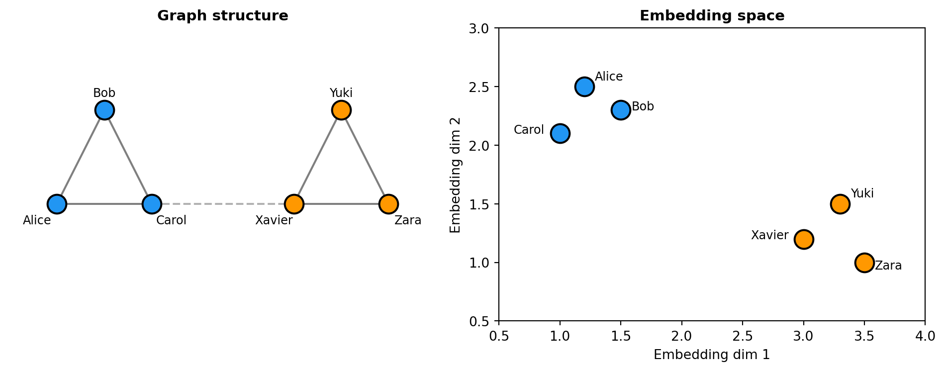
7.2 Visualizing Graph Embeddings

Figure 7.1: Graph embeddings: nodes in the same community (densely connected) map to nearby points in embedding space.

7.3 Creating Graph Embeddings

"""
Graph Embeddings: Network Structure as Vectors
"""

import numpy as np
from sklearn.metrics.pairwise import cosine_similarity

# Simulated node embeddings from a social network
# Real systems use Node2Vec, GraphSAGE, or GNN-based approaches
np.random.seed(42)

# Two friend groups: nodes in the same group have similar embeddings
node_embeddings = {
    # Community 1: Alice, Bob, Carol (densely connected)
    'Alice': np.random.randn(64) + np.array([1, 0] + [0]*62),
    'Bob': np.random.randn(64) + np.array([0.9, 0.1] + [0]*62),
    'Carol': np.random.randn(64) + np.array([0.8, 0.2] + [0]*62),
    # Community 2: Xavier, Yuki, Zara (densely connected)
    'Xavier': np.random.randn(64) + np.array([0, 1] + [0]*62),
    'Yuki': np.random.randn(64) + np.array([0.1, 0.9] + [0]*62),
    'Zara': np.random.randn(64) + np.array([0.2, 0.8] + [0]*62),
}

print("Graph embedding similarities:\n")
print("Within community (friends):")
ab = cosine_similarity([node_embeddings['Alice']], [node_embeddings['Bob']])[0][0]
ac = cosine_similarity([node_embeddings['Alice']], [node_embeddings['Carol']])[0][0]
print(f"  Alice ↔ Bob:   {ab:.3f}")
print(f"  Alice ↔ Carol: {ac:.3f}")

print("\nAcross communities (not connected):")
ax = cosine_similarity([node_embeddings['Alice']], [node_embeddings['Xavier']])[0][0]
print(f"  Alice ↔ Xavier: {ax:.3f}")

Graph embedding similarities:

Within community (friends):
  Alice ↔ Bob:   0.056
  Alice ↔ Carol: 0.000

Across communities (not connected):
  Alice ↔ Xavier: -0.035

Nodes in the same community have high similarity because they share connections. Alice, Bob, and Carol are all friends with each other, so their embeddings cluster together. Xavier is in a different friend group with no direct connection to Alice, resulting in lower similarity.

7.4 When to Use Graph Embeddings

When to use graph embeddings: Social network analysis (community detection, influence prediction, friend recommendation), recommendation systems with user-item graphs (see Chapter 13), knowledge graph completion to predict missing relationships (see Chapter 28), fraud detection to identify suspicious patterns in transaction graphs (see Chapter 29), drug discovery for molecule property prediction from molecular graphs (see Chapter 30), and supply chain analysis to identify dependencies and bottlenecks.

7.5 Popular Graph Architectures

Graph embedding architectures

Architecture	Type	Strengths	Use Cases
Node2Vec	Random walks	Simple, scalable	Homogeneous graphs
RDF2Vec	Random walks	Pre-trained KG models	RDF knowledge graphs
GraphSAGE	Neighborhood aggregation	Inductive learning	New nodes
GAT	Graph attention	Weighted neighbors	Heterogeneous graphs
TransE	Translation-based	Link prediction	Knowledge graphs

7.6 Advanced: How Graph Models Learn

NoteOptional Section

This section explains how graph embedding models learn structural patterns. Skip if you just need to use pre-built embeddings.

7.6.1 Node2Vec: Random Walks

Node2Vec (Mikolov et al. 2013) generates embeddings by performing random walks on the graph, then applying Word2Vec. The intuition: nodes that appear in similar “context” (nearby in random walks) should have similar embeddings.

def node2vec_walk(graph, start_node, walk_length, p=1, q=1):
    """Generate a random walk starting from a node."""
    walk = [start_node]
    while len(walk) < walk_length:
        cur = walk[-1]
        neighbors = list(graph.neighbors(cur))
        if len(neighbors) == 0:
            break
        # Biased sampling based on p (return) and q (in-out) parameters
        if len(walk) == 1:
            walk.append(random.choice(neighbors))
        else:
            prev = walk[-2]
            probs = []
            for neighbor in neighbors:
                if neighbor == prev:
                    probs.append(1/p)  # Return to previous
                elif graph.has_edge(neighbor, prev):
                    probs.append(1)  # Same neighborhood
                else:
                    probs.append(1/q)  # Explore
            probs = np.array(probs) / sum(probs)
            walk.append(np.random.choice(neighbors, p=probs))
    return walk

7.6.2 RDF2Vec: Knowledge Graph Embeddings

RDF2Vec (Ristoski and Paulheim 2016) adapts the Node2Vec approach for RDF knowledge graphs like DBpedia, Wikidata, and enterprise knowledge bases. Instead of treating nodes generically, it handles semantic triples (subject-predicate-object) and generates reusable entity embeddings.

The approach extracts random walks from knowledge graphs, optionally incorporating Weisfeiler-Lehman subtree patterns to capture richer structural information, then applies Word2Vec to learn embeddings. Unlike task-specific methods, RDF2Vec produces general-purpose entity vectors that can be reused across multiple downstream applications.

Key advantages:

• Pre-trained models available: KGvec2go hosts embeddings for DBpedia, Wikidata, WordNet, and other major knowledge graphs
• Incremental updates: Can adapt embeddings for graph updates without complete retraining
• Task-independent: Same embeddings work for classification, link prediction, similarity search, and other tasks
• Production-ready: PyRDF2Vec library provides easy implementation

When to use RDF2Vec:

• Entity classification in knowledge graphs
• Knowledge graph completion and link prediction
• Semantic search over structured enterprise data
• Integration with existing RDF/SPARQL infrastructure
• Applications requiring pre-computed embeddings from DBpedia or Wikidata

Resources:

• PyRDF2Vec library for implementation
• KGvec2go for pre-trained embeddings
• For comprehensive coverage, see Embedding Knowledge Graphs with RDF2vec (Paulheim, Portisch, and Ristoski 2023)

7.6.3 GraphSAGE: Neighborhood Aggregation

GraphSAGE learns embeddings by aggregating features from a node’s neighbors:

1. Sample a fixed number of neighbors for each node
2. Aggregate neighbor embeddings (mean, max, or LSTM)
3. Concatenate with the node’s own embedding
4. Apply a neural network layer

This is inductive: it can generate embeddings for new nodes not seen during training.

7.6.4 Graph Attention Networks (GAT)

GATs learn to weight neighbors differently based on their importance:

def gat_attention(node_emb, neighbor_embs, attention_weights):
    """Compute attention-weighted neighbor aggregation."""
    # Compute attention scores for each neighbor
    scores = []
    for neighbor_emb in neighbor_embs:
        combined = torch.cat([node_emb, neighbor_emb])
        score = torch.exp(attention_weights @ combined)
        scores.append(score)

    # Normalize to get attention weights
    attention = torch.softmax(torch.tensor(scores), dim=0)

    # Weighted aggregation
    aggregated = sum(a * emb for a, emb in zip(attention, neighbor_embs))
    return aggregated

7.7 Key Takeaways

• Graph embeddings capture network structure—connected nodes and nodes with similar neighborhoods have similar vectors
• The core principle: a node’s meaning comes from its connections, not just its features
• Random walks (Node2Vec) treat graphs like text, generating “sentences” of nodes to train Word2Vec
• Neighborhood aggregation (GraphSAGE, GAT) directly combines neighbor information, enabling inductive learning
• Applications span social networks, recommendations, fraud detection, and molecular property prediction

7.8 Looking Ahead

Now that you understand graph embeddings, Chapter 8 explores time-series embeddings—representations that capture temporal patterns and dynamics.

7.9 Further Reading

• Grover, A. & Leskovec, J. (2016). “node2vec: Scalable Feature Learning for Networks.” KDD
• Hamilton, W., et al. (2017). “Inductive Representation Learning on Large Graphs.” NeurIPS
• Veličković, P., et al. (2018). “Graph Attention Networks.” ICLR

Mikolov, Tomas, Kai Chen, Greg Corrado, and Jeffrey Dean. 2013. “Efficient Estimation of Word Representations in Vector Space.” arXiv Preprint arXiv:1301.3781.

Paulheim, Heiko, Jan Portisch, and Petar Ristoski. 2023. Embedding Knowledge Graphs with RDF2vec. Springer Nature. https://doi.org/10.1007/978-3-031-30387-6.

Ristoski, Petar, and Heiko Paulheim. 2016. “RDF2Vec: RDF Graph Embeddings for Data Mining.” In The Semantic Web–ISWC 2016: 15th International Semantic Web Conference, 498–514. Springer International Publishing; Springer.