2 Similarity and Distance Metrics
NoteChapter Overview
Choosing the right similarity or distance metric fundamentally affects embedding system performance. This chapter covers the major metrics—cosine similarity, Euclidean distance, dot product, and others—explaining when to use each, their mathematical properties, and practical implications for vector databases and retrieval quality.
2.1 Why Metric Choice Matters
The metric you choose determines:
- What “similar” means for your application
- Index performance in your vector database
- Retrieval quality for your use case
- Computational cost at query time
Different metrics capture different notions of similarity. Two embeddings might be “close” by one metric and “far” by another. Understanding these differences is essential for building effective embedding systems.
2.2 Cosine Similarity
We introduced cosine similarity briefly in Chapter 1; here we cover it in depth alongside other metrics so you can make informed choices.
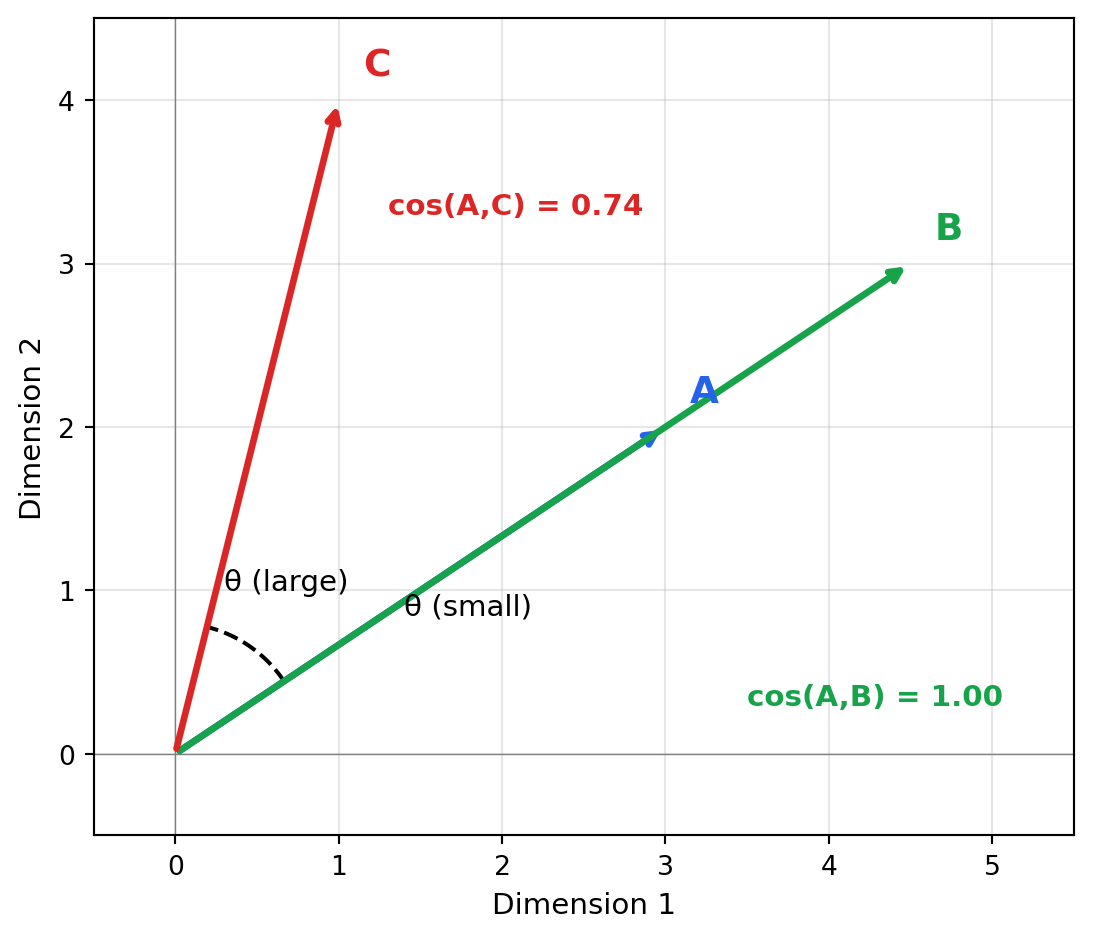
Think of cosine similarity as asking “are these vectors pointing in the same direction?” regardless of how long they are. Two documents about machine learning will point in a similar direction in embedding space whether one is a tweet or a textbook—their lengths differ, but their meaning aligns. This makes cosine similarity ideal for text, where document length shouldn’t affect semantic similarity.
Cosine similarity measures the angle between two vectors, ignoring their magnitudes:
\[\text{cosine\_similarity}(\mathbf{A}, \mathbf{B}) = \frac{\mathbf{A} \cdot \mathbf{B}}{||\mathbf{A}|| \times ||\mathbf{B}||} = \frac{\sum_{i=1}^{n} A_i B_i}{\sqrt{\sum_{i=1}^{n} A_i^2} \times \sqrt{\sum_{i=1}^{n} B_i^2}}\]
"""
Cosine Similarity: Angle-Based Comparison

Measures the cosine of the angle between vectors.
Range: -1 (opposite) to 1 (identical direction)
"""

import numpy as np
from scipy.spatial.distance import cosine

def cosine_similarity(a, b):
    """Calculate cosine similarity (1 = identical, -1 = opposite)."""
    return np.dot(a, b) / (np.linalg.norm(a) * np.linalg.norm(b))

# Example: Same direction, different magnitudes
v1 = np.array([1.0, 2.0, 3.0])
v2 = np.array([2.0, 4.0, 6.0])  # Same direction, 2x magnitude
v3 = np.array([3.0, 2.0, 1.0])  # Different direction

print("Cosine similarity examples:")
print(f"  v1 ↔ v2 (same direction, different magnitude): {cosine_similarity(v1, v2):.4f}")
print(f"  v1 ↔ v3 (different direction): {cosine_similarity(v1, v3):.4f}")
Cosine similarity examples:
v1 ↔ v2 (same direction, different magnitude): 1.0000
v1 ↔ v3 (different direction): 0.7143When to use cosine similarity:
- Text embeddings: Sentence transformers produce vectors where direction encodes meaning
- High-dimensional spaces (100+ dimensions): More stable than Euclidean distance
- When magnitude isn’t meaningful: Document length shouldn’t affect similarity
- Normalized embeddings: Most embedding models normalize output vectors
Cosine distance is simply 1 - cosine_similarity, converting similarity to distance where 0 = identical.
2.3 Euclidean Distance (L2)
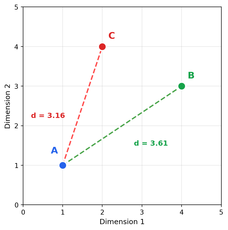
Think of Euclidean distance as “how far would I walk in a straight line?” It measures absolute position in space—if you plotted embeddings as points on a map, Euclidean distance is the crow-flies distance between them. Unlike cosine similarity, magnitude matters: a short document and a long document will be far apart even if they discuss identical topics, simply because their embedding magnitudes differ.
Euclidean distance measures the straight-line distance between two points:
\[\text{euclidean}(\mathbf{A}, \mathbf{B}) = \sqrt{\sum_{i=1}^{n} (A_i - B_i)^2} = ||\mathbf{A} - \mathbf{B}||_2\]
"""
Euclidean Distance: Straight-Line Distance

Measures absolute separation in space.
Range: 0 (identical) to infinity
"""

import numpy as np

def euclidean_distance(a, b):
    """Calculate Euclidean (L2) distance."""
    return np.linalg.norm(a - b)

# Same vectors as before
v1 = np.array([1.0, 2.0, 3.0])
v2 = np.array([2.0, 4.0, 6.0])  # Same direction, 2x magnitude
v3 = np.array([3.0, 2.0, 1.0])  # Different direction

print("Euclidean distance examples:")
print(f"  v1 ↔ v2 (same direction, different magnitude): {euclidean_distance(v1, v2):.4f}")
print(f"  v1 ↔ v3 (different direction): {euclidean_distance(v1, v3):.4f}")
print("\nNote: v1 and v2 are FAR by Euclidean but IDENTICAL by cosine!")
Euclidean distance examples:
v1 ↔ v2 (same direction, different magnitude): 3.7417
v1 ↔ v3 (different direction): 2.8284
Note: v1 and v2 are FAR by Euclidean but IDENTICAL by cosine!When to use Euclidean distance:
- Image embeddings: When pixel-level differences matter
- Low-dimensional spaces (< 50 dimensions): Works well
- When magnitude matters: Larger vectors should be “farther”
- Clustering applications: K-means uses Euclidean distance
Warning: Euclidean distance suffers from the curse of dimensionality. In high dimensions (768+), all points tend to become equidistant, reducing discriminative power.
2.4 Dot Product (Inner Product)
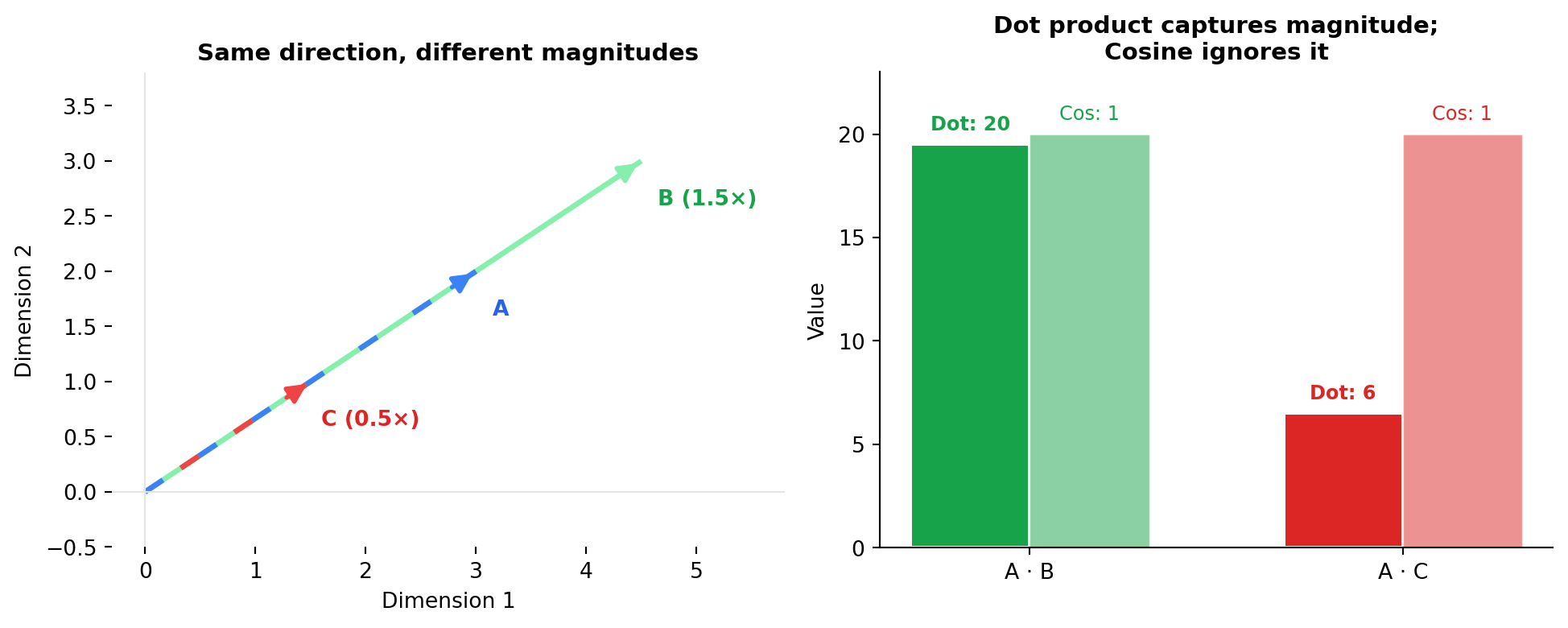
The dot product captures both direction and magnitude—think of it as “how much do these vectors agree, weighted by their strengths?” A user embedding strongly pointing toward “sci-fi” matched with a blockbuster sci-fi movie (large magnitude) scores higher than the same user matched with an obscure indie sci-fi film (small magnitude). This is why recommendation systems often use dot product: magnitude encodes confidence or importance.
The dot product is the unnormalized version of cosine similarity:
\[\text{dot\_product}(\mathbf{A}, \mathbf{B}) = \mathbf{A} \cdot \mathbf{B} = \sum_{i=1}^{n} A_i B_i\]
"""
Dot Product: Direction + Magnitude

Combines directional similarity with magnitude.
Range: -infinity to +infinity
"""

import numpy as np

def dot_product(a, b):
    """Calculate dot product."""
    return np.dot(a, b)

# Vectors with different magnitudes
v1 = np.array([1.0, 2.0, 3.0])
v2 = np.array([2.0, 4.0, 6.0])    # Same direction, 2x magnitude
v3 = np.array([0.5, 1.0, 1.5])    # Same direction, 0.5x magnitude

print("Dot product examples:")
print(f"  v1 · v1: {dot_product(v1, v1):.4f}")
print(f"  v1 · v2 (2x magnitude): {dot_product(v1, v2):.4f}")
print(f"  v1 · v3 (0.5x magnitude): {dot_product(v1, v3):.4f}")
print("\nDot product rewards both alignment AND magnitude")
Dot product examples:
v1 · v1: 14.0000
v1 · v2 (2x magnitude): 28.0000
v1 · v3 (0.5x magnitude): 7.0000
Dot product rewards both alignment AND magnitudeWhen to use dot product:
- Recommendation systems: User-item relevance often uses dot product scoring
- When magnitude encodes importance: Higher-magnitude vectors are “stronger” matches
- Maximum Inner Product Search (MIPS): Some vector DBs optimize for this
- Pre-normalized embeddings: Equivalent to cosine similarity when vectors are unit length
Relationship to cosine similarity: For unit-normalized vectors, dot product equals cosine similarity.
2.5 Manhattan Distance (L1)
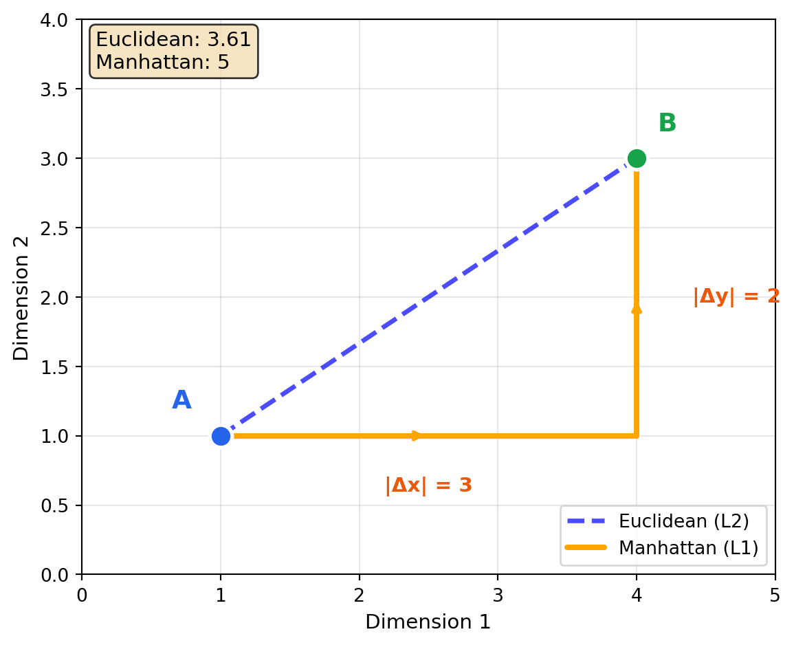
Imagine navigating a city grid—you can’t walk diagonally through buildings, only along streets. Manhattan distance measures how many blocks you’d walk: 3 blocks east plus 4 blocks north, not the 5-block diagonal shortcut. This axis-aligned measurement is more robust to outliers than Euclidean distance: one extreme dimension doesn’t dominate the total like it would when squared.
Manhattan distance sums the absolute differences along each dimension:
\[\text{manhattan}(\mathbf{A}, \mathbf{B}) = \sum_{i=1}^{n} |A_i - B_i| = ||\mathbf{A} - \mathbf{B}||_1\]
"""
Manhattan Distance: City-Block Distance

Sum of absolute differences along each axis.
Range: 0 (identical) to infinity
"""

import numpy as np

def manhattan_distance(a, b):
    """Calculate Manhattan (L1) distance."""
    return np.sum(np.abs(a - b))

v1 = np.array([1.0, 2.0, 3.0])
v2 = np.array([4.0, 6.0, 3.0])

euclidean = np.linalg.norm(v1 - v2)
manhattan = manhattan_distance(v1, v2)

print("Comparing L1 vs L2 distance:")
print(f"  Euclidean (L2): {euclidean:.4f}")
print(f"  Manhattan (L1): {manhattan:.4f}")
Comparing L1 vs L2 distance:
Euclidean (L2): 5.0000
Manhattan (L1): 7.0000When to use Manhattan distance:
- Sparse data: Less sensitive to outliers than Euclidean
- Grid-like domains: When movement is constrained to axes
- Feature independence: When dimensions represent independent attributes
- Robust similarity: Less affected by a single large difference
2.6 Hamming Distance
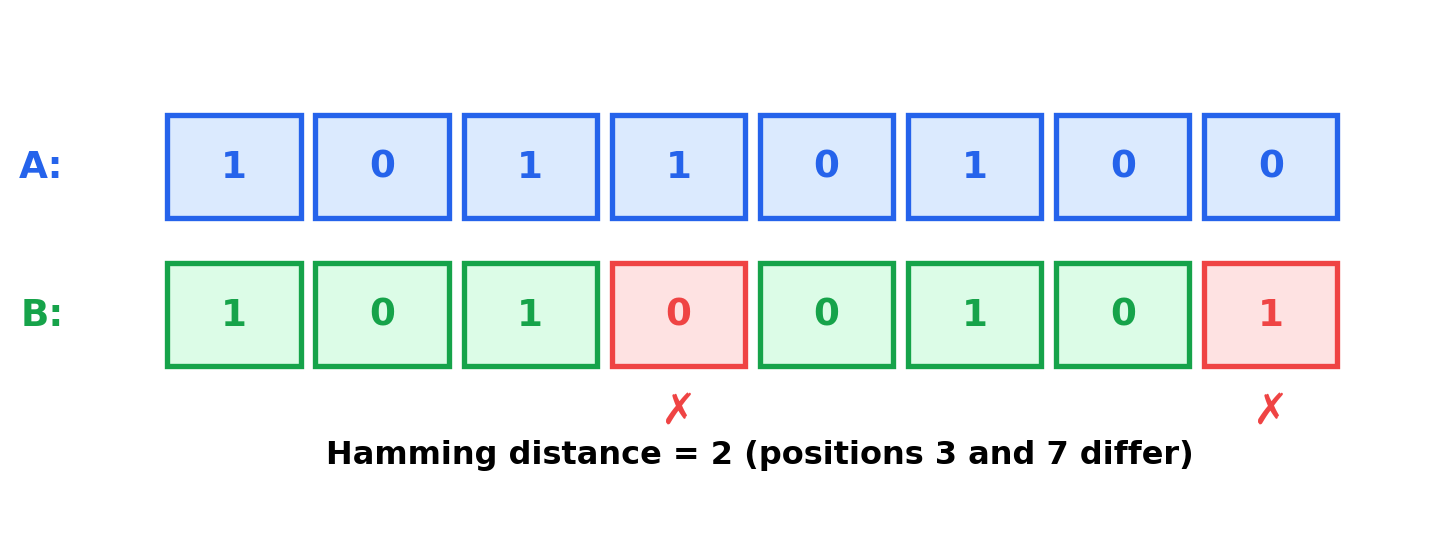
Hamming distance answers a simple question: “how many bits need to flip to transform one vector into the other?” If you compress embeddings to binary codes (0s and 1s), comparing them becomes blazingly fast—just XOR the bit strings and count the 1s. This makes Hamming distance essential for billion-scale search where you trade some accuracy for 32× storage savings and hardware-accelerated comparison.
Hamming distance counts the number of positions where values differ. For binary embeddings:
\[\text{hamming}(\mathbf{A}, \mathbf{B}) = \sum_{i=1}^{n} \mathbf{1}[A_i \neq B_i]\]
"""
Hamming Distance: Bit-Level Comparison

Counts positions where values differ.
Essential for binary/quantized embeddings.
"""

import numpy as np

def hamming_distance(a, b):
    """Calculate Hamming distance for binary vectors."""
    return np.sum(a != b)

def hamming_similarity(a, b):
    """Normalized Hamming similarity (0 to 1)."""
    return 1 - hamming_distance(a, b) / len(a)

# Binary embeddings (e.g., from quantization)
b1 = np.array([1, 0, 1, 1, 0, 1, 0, 0])
b2 = np.array([1, 0, 1, 0, 0, 1, 0, 1])  # 2 bits different
b3 = np.array([0, 1, 0, 0, 1, 0, 1, 1])  # 8 bits different

print("Hamming distance (binary embeddings):")
print(f"  b1 ↔ b2 (similar): {hamming_distance(b1, b2)} bits differ, similarity: {hamming_similarity(b1, b2):.3f}")
print(f"  b1 ↔ b3 (opposite): {hamming_distance(b1, b3)} bits differ, similarity: {hamming_similarity(b1, b3):.3f}")
Hamming distance (binary embeddings):
b1 ↔ b2 (similar): 2 bits differ, similarity: 0.750
b1 ↔ b3 (opposite): 8 bits differ, similarity: 0.000When to use Hamming distance:
- Binary embeddings: From binarization or locality-sensitive hashing
- Quantized vectors: After product quantization
- Extreme scale: Binary comparison is very fast (XOR + popcount)
- Memory-constrained: Binary vectors use 32x less storage than float32
See Section 10.7 for more on binary and quantized embeddings.
2.7 Jaccard Similarity
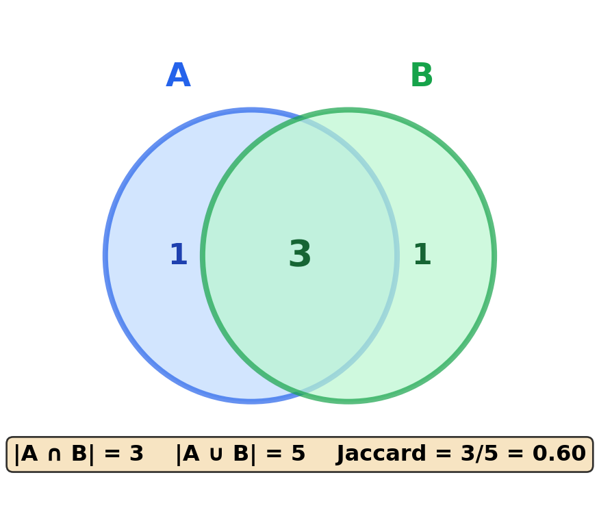
Jaccard similarity asks “what fraction of items do these two sets share?” If two users have watched 10 movies total between them, and 6 of those are the same, their Jaccard similarity is 6/10 = 0.6. It’s intuitive for sparse, binary features like tags, categories, or bag-of-words representations where you care about presence/absence rather than counts or magnitudes.
Jaccard similarity measures overlap between sets:
\[\text{jaccard}(\mathbf{A}, \mathbf{B}) = \frac{|A \cap B|}{|A \cup B|}\]
"""
Jaccard Similarity: Set Overlap

Measures intersection over union.
Range: 0 (no overlap) to 1 (identical sets)
"""

import numpy as np

def jaccard_similarity(a, b):
    """Calculate Jaccard similarity for binary/set vectors."""
    intersection = np.sum(np.logical_and(a, b))
    union = np.sum(np.logical_or(a, b))
    return intersection / union if union > 0 else 0

# Binary feature vectors (e.g., document has word or not)
doc1 = np.array([1, 1, 1, 0, 0, 1, 0, 0])  # Has words: 0, 1, 2, 5
doc2 = np.array([1, 1, 0, 0, 0, 1, 1, 0])  # Has words: 0, 1, 5, 6
doc3 = np.array([0, 0, 0, 1, 1, 0, 0, 1])  # Has words: 3, 4, 7

print("Jaccard similarity (set overlap):")
print(f"  doc1 ↔ doc2 (3 shared, 5 total): {jaccard_similarity(doc1, doc2):.3f}")
print(f"  doc1 ↔ doc3 (0 shared): {jaccard_similarity(doc1, doc3):.3f}")
Jaccard similarity (set overlap):
doc1 ↔ doc2 (3 shared, 5 total): 0.600
doc1 ↔ doc3 (0 shared): 0.000When to use Jaccard similarity:
- Sparse binary features: Bag-of-words, tag sets
- Set membership: When presence/absence matters, not magnitude
- Near-duplicate detection: MinHash approximates Jaccard efficiently
- Categorical data: When features are one-hot encoded
2.8 Metric Comparison Summary
| Metric | Range | Magnitude Sensitive | Best For | Vector DB Support |
|---|---|---|---|---|
| Cosine | -1 to 1 | No | Text, normalized embeddings | Universal |
| Euclidean (L2) | 0 to ∞ | Yes | Images, low-dimensional | Universal |
| Dot Product | -∞ to ∞ | Yes | Recommendations, MIPS | Most |
| Manhattan (L1) | 0 to ∞ | Yes | Sparse data, outlier-robust | Some |
| Hamming | 0 to n | N/A (binary) | Binary embeddings | Some |
| Jaccard | 0 to 1 | N/A (sets) | Sparse sets, tags | Limited |
2.9 Choosing the Right Metric
| Use Case | Embedding Type | Normalized? | Recommended Metric |
|---|---|---|---|
| Text (sentence transformers) | Dense | Yes | Cosine / Dot product |
| Image (CNN features) | Dense | No | Dot product |
| Recommendations (user-item) | Dense | No | Dot product |
| Binary hash codes | Binary | N/A | Hamming |
| Document tags | Sparse binary | N/A | Jaccard |
2.9.1 Decision Tree
Is your embedding binary?
├── Yes → Hamming distance
└── No → Is it sparse binary (sets/tags)?
    ├── Yes → Jaccard similarity
    └── No → Are vectors normalized?
        ├── Yes → Cosine similarity (fastest)
        └── No → Does magnitude encode importance?
            ├── Yes → Dot product or Euclidean
            └── No → Cosine similarity
2.10 Impact on Vector Database Performance
Your metric choice affects index structure, query latency, and storage requirements:
| Metric | Index Type | HNSW Support | Storage | Query Overhead |
|---|---|---|---|---|
| Cosine | Normalize + L2 | ✓ Native | 1x | Normalize query |
| Euclidean (L2) | Native L2 | ✓ Native | 1x | None |
| Dot Product | MIPS or augmented L2 | ✓ With transform | 1x-1.01x | May need augmentation |
| Hamming | Binary index | Specialized | 0.03x (32x smaller) | Bitwise ops only |
2.10.1 Why This Matters
Cosine vs. L2 equivalence: For normalized vectors, cosine similarity and L2 distance produce identical rankings. Most databases exploit this—they normalize vectors once at insertion, then use fast L2 indexes:
# These produce the same ranking for normalized vectors:
# cosine_sim(a, b) = 1 - (L2_dist(a, b)² / 2)
Dot product challenges: Unlike cosine and L2, dot product (MIPS—Maximum Inner Product Search) doesn’t satisfy the triangle inequality. Some databases handle this by:
- Appending a dimension to convert MIPS → L2 (slight storage overhead)
- Using specialized MIPS indexes (less common)
Binary embeddings: Hamming distance enables 32x storage reduction (float32 → 1 bit per dimension) with specialized binary indexes. Ideal for large-scale deduplication where some quality loss is acceptable.
TipPerformance Tip
If using cosine similarity, pre-normalize your embeddings before insertion. This avoids redundant normalization at query time and lets you use faster L2 indexes directly.
2.11 Practical Considerations
2.11.1 Normalization
"""
L2 Normalization: Making Cosine = Dot Product
"""

import numpy as np

def l2_normalize(vectors):
    """Normalize vectors to unit length."""
    norms = np.linalg.norm(vectors, axis=1, keepdims=True)
    return vectors / norms

# Original vectors
vectors = np.array([
    [3.0, 4.0],      # Magnitude 5
    [1.0, 1.0],      # Magnitude √2
    [10.0, 0.0],     # Magnitude 10
])

normalized = l2_normalize(vectors)

print("Before normalization:")
print(f"  Magnitudes: {np.linalg.norm(vectors, axis=1)}")

print("\nAfter L2 normalization:")
print(f"  Magnitudes: {np.linalg.norm(normalized, axis=1)}")

# Now dot product = cosine similarity
v1, v2 = normalized[0], normalized[1]
dot = np.dot(v1, v2)
cos = np.dot(v1, v2) / (np.linalg.norm(v1) * np.linalg.norm(v2))
print(f"\nFor normalized vectors: dot product = {dot:.4f}, cosine = {cos:.4f}")
Before normalization:
Magnitudes: [ 5. 1.41421356 10. ]
After L2 normalization:
Magnitudes: [1. 1. 1.]
For normalized vectors: dot product = 0.9899, cosine = 0.98992.11.2 Metric Selection by Domain
| Domain | Typical Metric | Reason |
|---|---|---|
| Semantic search | Cosine | Text embeddings are normalized |
| Image retrieval | Cosine or L2 | Depends on model output |
| Recommendations | Dot product | Magnitude = confidence |
| Face recognition | Cosine | Normalized face embeddings |
| Document dedup | Jaccard or Cosine | Depending on representation |
| Binary codes | Hamming | Fast bitwise operations |
2.12 Emerging and Future Metrics
The standard metrics above handle most use cases, but research continues to develop specialized approaches for challenging scenarios.
2.12.1 Hyperbolic Distance
For hierarchical data (taxonomies, org charts, knowledge graphs), Euclidean space is inefficient—it can’t naturally represent tree structures. Hyperbolic space has negative curvature that matches hierarchical growth patterns:
"""
Hyperbolic Distance (Poincaré Ball Model)

Hyperbolic space naturally represents hierarchies.
Points near the center are "general"; points near the edge are "specific".
"""

import numpy as np

def poincare_distance(u, v):
    """
    Distance in the Poincaré ball model of hyperbolic space.

    As points approach the boundary (norm → 1), distances grow rapidly,
    creating "room" for exponentially many nodes at each level.
    """
    norm_u_sq = np.sum(u ** 2)
    norm_v_sq = np.sum(v ** 2)
    norm_diff_sq = np.sum((u - v) ** 2)

    # Hyperbolic distance formula
    return np.arccosh(
        1 + 2 * norm_diff_sq / ((1 - norm_u_sq) * (1 - norm_v_sq))
    )

# Example: Points in 2D Poincaré ball
center = np.array([0.0, 0.0])      # Root of hierarchy
mid_level = np.array([0.5, 0.0])   # Middle of tree
leaf = np.array([0.9, 0.0])        # Leaf node (near boundary)

print("Hyperbolic distances (Poincaré ball):")
print(f"  Center ↔ Mid-level: {poincare_distance(center, mid_level):.3f}")
print(f"  Mid-level ↔ Leaf: {poincare_distance(mid_level, leaf):.3f}")
print(f"  Center ↔ Leaf: {poincare_distance(center, leaf):.3f}")
Hyperbolic distances (Poincaré ball):
Center ↔ Mid-level: 1.099
Mid-level ↔ Leaf: 1.846
Center ↔ Leaf: 2.944Use cases: Product taxonomies, organizational hierarchies, knowledge graphs. Hyperbolic embeddings can represent hierarchies in 5-20 dimensions that would require 100-500 dimensions in Euclidean space.
2.12.2 Learned Similarity Functions
Instead of choosing a fixed metric, learn the similarity function from your data:
"""
Learned Similarity: Let the model decide what "similar" means.

Approaches:
1. Mahalanobis distance (learns covariance structure)
2. Siamese networks (learn embedding + comparison jointly)
3. Cross-encoders (attend across both inputs)
"""

import numpy as np

class LearnedMahalanobis:
    """
    Mahalanobis distance with learned transformation matrix.

    Learns which dimensions matter and how they correlate.
    Equivalent to: d(x,y) = sqrt((x-y)^T M (x-y)) where M is learned.
    """

    def __init__(self, dim):
        # Initialize as identity (reduces to Euclidean)
        self.L = np.eye(dim)  # M = L^T L ensures positive semi-definite

    def distance(self, x, y):
        """Compute Mahalanobis distance with learned metric."""
        diff = x - y
        transformed = self.L @ diff
        return np.sqrt(np.sum(transformed ** 2))

    def fit(self, similar_pairs, dissimilar_pairs, learning_rate=0.01):
        """
        Learn metric from supervision (simplified).
        Real implementation uses gradient descent on triplet/contrastive loss.
        """
        # Pull similar pairs closer, push dissimilar pairs apart
        pass  # Actual training loop omitted for brevity

# Example usage
metric = LearnedMahalanobis(dim=128)
x = np.random.randn(128)
y = np.random.randn(128)
print(f"Learned Mahalanobis distance: {metric.distance(x, y):.3f}")
Learned Mahalanobis distance: 16.261When to use learned metrics: - Domain-specific similarity (what’s “similar” in your domain isn’t captured by cosine) - Few-shot learning (learn from limited examples) - When you have supervision signal (click data, ratings, labels)
2.12.3 Approximate Metrics at Scale
At billion-scale, even computing exact similarity becomes expensive. Approximate metrics trade accuracy for speed:
"""
Approximate Similarity for Extreme Scale

Techniques:
1. Locality-Sensitive Hashing (LSH): Hash similar items to same bucket
2. Product Quantization (PQ): Compress vectors, approximate distance
3. Random Projections: Preserve relative distances approximately
"""

import numpy as np

def random_projection_similarity(a, b, n_projections=100, seed=42):
    """
    Approximate cosine similarity using random projections.

    Project to random hyperplanes, count sign agreements.
    More agreements = more similar (probabilistically).
    """
    np.random.seed(seed)
    dim = len(a)

    # Generate random projection vectors
    projections = np.random.randn(n_projections, dim)

    # Project both vectors
    proj_a = np.sign(projections @ a)
    proj_b = np.sign(projections @ b)

    # Count agreements (same sign = similar direction)
    agreement_rate = np.mean(proj_a == proj_b)

    # Convert to approximate cosine similarity
    # (1 - 2*theta/pi) where theta is angle
    approx_cosine = np.cos(np.pi * (1 - agreement_rate))

    return approx_cosine

# Compare exact vs approximate
a = np.random.randn(768)
b = a + np.random.randn(768) * 0.5  # Similar vector

exact_cosine = np.dot(a, b) / (np.linalg.norm(a) * np.linalg.norm(b))
approx_cosine = random_projection_similarity(a, b)

print("Exact vs Approximate similarity:")
print(f"  Exact cosine: {exact_cosine:.4f}")
print(f"  Approx (100 projections): {approx_cosine:.4f}")
print(f"  Error: {abs(exact_cosine - approx_cosine):.4f}")
Exact vs Approximate similarity:
Exact cosine: 0.8827
Approx (100 projections): 0.7705
Error: 0.1122Trade-offs: - LSH: O(1) lookup but requires tuning hash functions - PQ: 10-100x compression, ~5% recall loss typical - Random projections: Simple, parallelizable, theoretical guarantees
2.12.4 Task-Adaptive Metrics
The best metric depends on your task. Metric learning optimizes the similarity function end-to-end:
| Approach | How It Works | Best For |
|---|---|---|
| Triplet loss | Learn: d(anchor, positive) < d(anchor, negative) | Face recognition, retrieval |
| Contrastive loss | Pull positives together, push negatives apart | Self-supervised learning |
| Cross-encoder | Jointly encode both inputs, predict similarity | Reranking, high-precision |
| Late interaction | Multiple vectors per item, aggregate similarities | Fine-grained matching |
For detailed coverage of these training approaches, see Chapter 15 and Chapter 16.
2.13 Key Takeaways
Cosine similarity is the default for most embedding applications—it ignores magnitude and works well in high dimensions
Euclidean distance is magnitude-sensitive and works best in lower dimensions; suffers from curse of dimensionality at 768+ dims
Dot product rewards both alignment and magnitude—use when larger embeddings should match more strongly
Hamming distance enables ultra-fast search on binary embeddings with 32x storage savings
Metric choice affects indexing: Most vector databases optimize for L2/cosine; other metrics may require transformation
Pre-normalize for cosine: If using cosine similarity, normalize vectors before insertion to avoid redundant computation
Emerging approaches like hyperbolic distance, learned metrics, and approximate similarity address specialized needs—hierarchical data, domain-specific similarity, and extreme scale
2.14 Looking Ahead
With similarity metrics understood, Chapter 3 covers how vector databases use these metrics to build efficient indexes at scale. For binary and quantized embeddings that use Hamming distance, see Section 10.7 in the advanced patterns chapter.
2.15 Further Reading
- Aggarwal, C. C., Hinneburg, A., & Keim, D. A. (2001). “On the Surprising Behavior of Distance Metrics in High Dimensional Space.” ICDT
- Johnson, J., Douze, M., & Jégou, H. (2019). “Billion-scale similarity search with GPUs.” IEEE Transactions on Big Data
- Wang, J., et al. (2018). “A Survey on Learning to Hash.” IEEE TPAMI