This chapter covers text embeddings—the most mature and widely used embedding type. We explore what text embeddings are, when to use them, and the practical applications they enable. An optional advanced section explains how the underlying models learn to create these representations.
4.1 What Are Text Embeddings?
Text embeddings convert words, sentences, or documents into dense numerical vectors that capture semantic meaning. Unlike simple approaches like bag-of-words or TF-IDF, embeddings understand that “happy” and “joyful” are related, even though they share no letters.
The key insight: text that appears in similar contexts should have similar embeddings. This emerges from training on massive text corpora where the model learns to predict words from their surrounding context.
4.2 Word Embeddings
The foundation of modern NLP, word embeddings map individual words to vectors:
"""Word Embeddings: From Words to VectorsWord embeddings capture semantic relationships between individual words.Words with similar meanings cluster together in the embedding space."""import osos.environ["TOKENIZERS_PARALLELISM"] ="false"from sentence_transformers import SentenceTransformerfrom sklearn.metrics.pairwise import cosine_similarityimport numpy as np# Use a sentence model to embed individual wordsmodel = SentenceTransformer('all-MiniLM-L6-v2')# Embed words across different categorieswords = {'animals': ['cat', 'dog', 'elephant', 'whale'],'vehicles': ['car', 'truck', 'airplane', 'boat'],'colors': ['red', 'blue', 'green', 'yellow'],}all_words = [w for group in words.values() for w in group]embeddings = model.encode(all_words)# Show that words cluster by categoryprint("Word similarities (same category = higher similarity):\n")print("Within categories:")print(f" cat ↔ dog: {cosine_similarity([embeddings[0]], [embeddings[1]])[0][0]:.3f}")print(f" car ↔ truck: {cosine_similarity([embeddings[4]], [embeddings[5]])[0][0]:.3f}")print(f" red ↔ blue: {cosine_similarity([embeddings[8]], [embeddings[9]])[0][0]:.3f}")print("\nAcross categories:")print(f" cat ↔ car: {cosine_similarity([embeddings[0]], [embeddings[4]])[0][0]:.3f}")print(f" dog ↔ red: {cosine_similarity([embeddings[1]], [embeddings[8]])[0][0]:.3f}")
Word similarities (same category = higher similarity):

Within categories:
  cat ↔ dog:      0.661
  car ↔ truck:    0.689
  red ↔ blue:     0.729

Across categories:
  cat ↔ car:      0.463
  dog ↔ red:      0.377
Key characteristics:
One vector per word (static, context-independent in classic models)
Typically 100-300 dimensions
Captures synonyms, analogies, and semantic relationships
4.3 Sentence and Document Embeddings
Modern applications need to embed entire sentences or documents:
"""Sentence Embeddings: Capturing Complete ThoughtsSentence embeddings represent the meaning of entire sentences,enabling semantic search and similarity comparison."""from sentence_transformers import SentenceTransformerfrom sklearn.metrics.pairwise import cosine_similaritymodel = SentenceTransformer('all-MiniLM-L6-v2')# Sentences with similar meaning but different wordssentences = ["The quick brown fox jumps over the lazy dog","A fast auburn fox leaps above a sleepy canine","Machine learning models require lots of training data","AI systems need substantial amounts of examples to learn",]embeddings = model.encode(sentences)print("Sentence similarities:\n")print("Similar meaning (paraphrases):")print(f" Sentence 1 ↔ 2: {cosine_similarity([embeddings[0]], [embeddings[1]])[0][0]:.3f}")print(f" Sentence 3 ↔ 4: {cosine_similarity([embeddings[2]], [embeddings[3]])[0][0]:.3f}")print("\nDifferent topics:")print(f" Sentence 1 ↔ 3: {cosine_similarity([embeddings[0]], [embeddings[2]])[0][0]:.3f}")
Sentence similarities:

Similar meaning (paraphrases):
  Sentence 1 ↔ 2: 0.733
  Sentence 3 ↔ 4: 0.525

Different topics:
  Sentence 1 ↔ 3: -0.024
4.4 When to Use Text Embeddings
Text embeddings are the right choice for:
Text classification, clustering, and sentiment analysis (see Section 4.6)
Question answering and RAG systems (see Chapter 11)
Chatbots and conversational AI—intent matching, response selection (see Section 11.6)
Summarization—finding representative sentences (see Section 11.7)
Semantic search—finding documents by meaning (see Chapter 12)
Recommendation systems—content-based filtering (see Chapter 13)
Customer support—ticket routing, finding similar issues (see Chapter 26)
Content moderation—detecting similar problematic content (see Section 26.7)
Duplicate and near-duplicate detection (see Chapter 28)
Entity resolution—matching names and descriptions (see Chapter 28)
Machine translation—cross-lingual embeddings (see Chapter 35)
4.6 Classification, Clustering, and Sentiment Analysis
Once you have text embeddings, three foundational tasks become straightforward: classification (assigning labels), clustering (discovering groups), and sentiment analysis (a special case of classification). All three leverage the same principle—similar texts have similar embeddings.
Classification with embeddings:
Train a simple classifier on top of frozen embeddings, or use nearest-neighbor approaches. The k-NN (k-nearest neighbors) method shown below works as follows: during training, embed each text and store the embedding alongside its label. To predict a new text’s label, embed it, find the k training embeddings most similar to it (using cosine similarity), and return the most common label among those neighbors.
Show Text Classifier
import numpy as npfrom collections import Counterclass EmbeddingClassifier:"""Simple k-NN classifier using embeddings."""def__init__(self, encoder, k: int=5):self.encoder = encoderself.k = kself.embeddings = []self.labels = []def fit(self, texts: list, labels: list):"""Embed texts and store with their labels."""self.embeddings = [self.encoder.encode(text) for text in texts]self.labels = labelsdef predict(self, text: str) ->str:"""Predict label using k-NN.""" query_emb =self.encoder.encode(text)# Cosine similarity: (A · B) / (||A|| × ||B||) distances = []for i, emb inenumerate(self.embeddings): dist = np.dot(query_emb, emb) / (np.linalg.norm(query_emb) * np.linalg.norm(emb)) distances.append((dist, self.labels[i]))# Get k nearest neighbors distances.sort(reverse=True) k_nearest = [label for _, label in distances[: self.k]]# Return most common labelreturn Counter(k_nearest).most_common(1)[0][0]# Example: Sentiment classificationfrom sentence_transformers import SentenceTransformerencoder = SentenceTransformer('all-MiniLM-L6-v2')classifier = EmbeddingClassifier(encoder, k=3)classifier.fit( texts=["Great product!", "Loved it", "Terrible", "Waste of money", "Amazing quality"], labels=["positive", "positive", "negative", "negative", "positive"],)print(f"Prediction for 'This is wonderful!': {classifier.predict('This is wonderful!')}")
Prediction for 'This is wonderful!': positive
TipClassification Best Practices
Few-shot is often enough: With good embeddings, 10-50 examples per class often suffices (see Chapter 16 for few-shot techniques)
k-NN for simplicity: No training required, just store examples
Logistic regression for speed: Train a simple linear classifier on embeddings
Fine-tune for best quality: When you have thousands of examples, fine-tune the embedding model itself (see Chapter 14)
Clustering with embeddings:
Clustering discovers natural groups in your data without predefined labels. Since similar texts have similar embeddings, texts on the same topic will cluster together in embedding space.
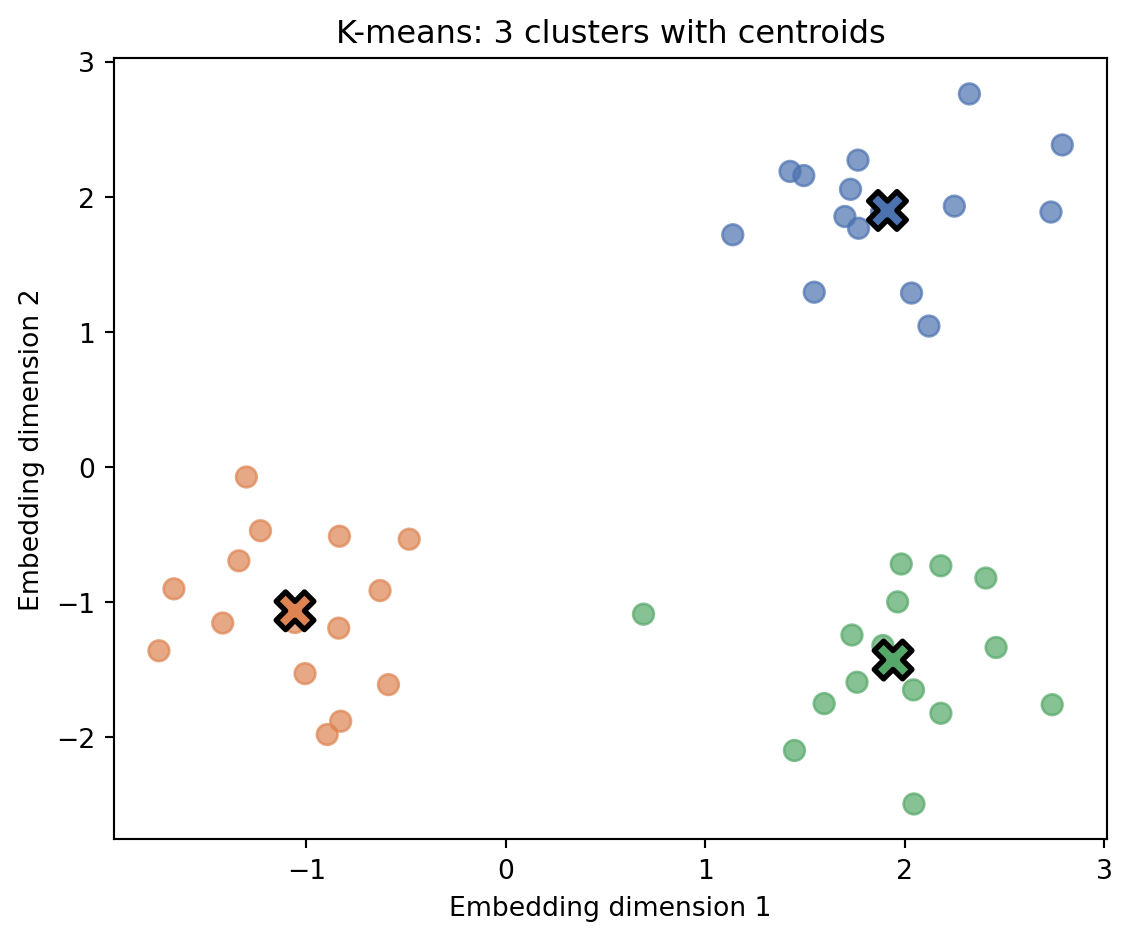
K-means is a popular clustering algorithm. You specify k (the number of clusters), and the algorithm finds k groups by positioning a centroid (center point) for each cluster. Each text belongs to the cluster whose centroid is closest to its embedding.
The algorithm works as follows: first, embed all texts. Then pick k random embeddings as initial centroids—the algorithm needs starting points before it can begin refining. Next, iterate until convergence: (1) assign each embedding to its nearest centroid (measured by Euclidean distance), and (2) update each centroid to be the mean of its assigned embeddings. The algorithm converges when assignments stop changing.
Figure 4.1: K-means clustering in 2D embedding space. Points are colored by cluster assignment, with centroids marked as X.
Show Text Clustering
import numpy as npfrom typing import List, Dictclass EmbeddingClusterer:"""K-means clustering on text embeddings."""def__init__(self, encoder, n_clusters: int=3):self.encoder = encoderself.n_clusters = n_clustersself.centroids =Nonedef fit(self, texts: List[str], max_iters: int=100):"""Cluster texts and return assignments.""" embeddings = np.array([self.encoder.encode(text) for text in texts])# Initialize centroids by picking k random embeddings as starting points indices = np.random.choice(len(embeddings), self.n_clusters, replace=False)self.centroids = embeddings[indices].copy()for _ inrange(max_iters):# Assign points to nearest centroid assignments = []for emb in embeddings: distances = [np.linalg.norm(emb - c) for c inself.centroids] assignments.append(np.argmin(distances))# Update centroids new_centroids = []for i inrange(self.n_clusters): cluster_points = embeddings[np.array(assignments) == i]iflen(cluster_points) >0: new_centroids.append(cluster_points.mean(axis=0))else: new_centroids.append(self.centroids[i])self.centroids = np.array(new_centroids)return assignmentsdef get_cluster_examples(self, texts: List[str], assignments: List[int]) -> Dict[int, List[str]]:"""Group texts by cluster.""" clusters = {i: [] for i inrange(self.n_clusters)}for text, cluster_id inzip(texts, assignments): clusters[cluster_id].append(text)return clusters# Example: Topic discoverytexts = [# Cooking"Chop the onions and garlic finely","Simmer the sauce for twenty minutes","Season with salt and pepper to taste","Preheat the oven to 350 degrees",# Space"The telescope discovered a new exoplanet","Astronauts completed their spacewalk today","The Mars rover collected soil samples","A new comet is visible this month",# Weather"Heavy rain expected throughout the weekend","Temperatures will drop below freezing tonight","A warm front is moving in from the south","Clear skies and sunshine forecast for Monday",]np.random.seed(42) # For reproducible resultsclusterer = EmbeddingClusterer(encoder, n_clusters=3)assignments = clusterer.fit(texts)clusters = clusterer.get_cluster_examples(texts, assignments)for cluster_id, examples in clusters.items():print(f"\nCluster {cluster_id}:")for text in examples:print(f" - {text}")
Cluster 0:
  - The Mars rover collected soil samples
  - A new comet is visible this month
  - A warm front is moving in from the south

Cluster 1:
  - Preheat the oven to 350 degrees
  - Astronauts completed their spacewalk today
  - Heavy rain expected throughout the weekend
  - Temperatures will drop below freezing tonight
  - Clear skies and sunshine forecast for Monday

Cluster 2:
  - Chop the onions and garlic finely
  - Simmer the sauce for twenty minutes
  - Season with salt and pepper to taste
  - The telescope discovered a new exoplanet
Notice that some items may appear in unexpected clusters. Embeddings capture semantic similarity that doesn’t always match our intuitive topic categories—“Preheat the oven to 350 degrees” mentions temperature, which may pull it toward weather texts, while “A warm front is moving in” uses directional language similar to space descriptions. This is a feature, not a bug: embeddings capture meaning patterns that humans might overlook.
TipClustering Best Practices
Choose k carefully: Use elbow method or silhouette scores to find optimal cluster count
HDBSCAN for unknown k: Unlike k-means, HDBSCAN doesn’t require specifying cluster count upfront—it discovers clusters based on density and labels sparse points as outliers rather than forcing them into clusters
Reduce dimensions first: For visualization, use UMAP or t-SNE on embeddings
Label clusters post-hoc: Examine cluster members to assign meaningful names
Sentiment analysis:
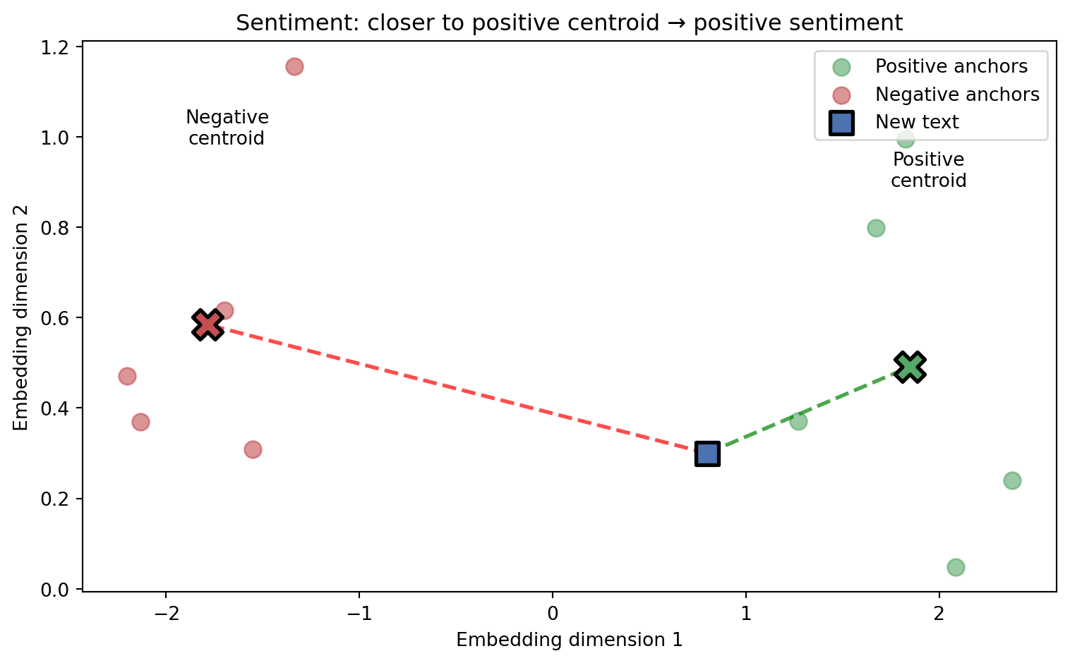
Sentiment analysis determines whether text expresses positive, negative, or neutral opinions. While you could treat this as classification (train on labeled examples), an elegant alternative uses anchor texts—words or phrases with known sentiment.
The approach works as follows: embed a set of clearly positive words (“excellent”, “amazing”, “love it”) and compute their centroid. Do the same for negative words. To analyze new text, embed it and measure which centroid it’s closer to. The difference in distances gives both a label and a confidence score—text much closer to the positive centroid is strongly positive.
Figure 4.2: Sentiment analysis using anchor texts. Positive and negative anchor words form centroids. New text is classified by which centroid it’s closer to.
Show Sentiment Analyzer
import numpy as npfrom typing import Tupleclass SentimentAnalyzer:"""Embedding-based sentiment analysis using anchor texts."""def__init__(self, encoder):self.encoder = encoder# Anchor texts define the sentiment space positive_anchors = ["excellent", "amazing", "wonderful", "fantastic", "love it"] negative_anchors = ["terrible", "awful", "horrible", "hate it", "worst ever"]# Compute anchor centroids: average the embeddings of all anchor words# to find the "center" of positive/negative regions in embedding space.# Using multiple anchors makes the centroid more robust than any single word.self.positive_centroid = np.mean( [encoder.encode(t) for t in positive_anchors], axis=0 )self.negative_centroid = np.mean( [encoder.encode(t) for t in negative_anchors], axis=0 )def analyze(self, text: str) -> Tuple[str, float]:""" Return sentiment label and confidence score. Score ranges from -1 (negative) to +1 (positive). """ emb =self.encoder.encode(text)# Cosine similarity: (A · B) / (||A|| × ||B||) pos_sim = np.dot(emb, self.positive_centroid) / ( np.linalg.norm(emb) * np.linalg.norm(self.positive_centroid) ) neg_sim = np.dot(emb, self.negative_centroid) / ( np.linalg.norm(emb) * np.linalg.norm(self.negative_centroid) )# Score: positive if closer to positive centroid score = pos_sim - neg_sim label ="positive"if score >0else"negative" confidence =abs(score)return label, confidence# Example usagenp.random.seed(42)analyzer = SentimentAnalyzer(encoder)for text in ["This product exceeded expectations!", "Complete waste of money"]: label, conf = analyzer.analyze(text)print(f"'{text[:30]}...' -> {label} ({conf:.2f})")
The number in parentheses is the confidence score—the difference between cosine similarities to the positive and negative centroids. These values appear low because general-purpose embeddings capture broad semantics, not just sentiment. The key insight is that the relative scores still correctly distinguish positive from negative text, even when absolute differences are small. For production sentiment analysis, you’d typically fine-tune embeddings on sentiment-labeled data (see Chapter 14).
TipSentiment Analysis Best Practices
Domain matters: Financial sentiment differs from product reviews—use domain-specific anchors (see Chapter 29 for financial sentiment)
Beyond binary: Instead of just positive/negative centroids, create centroids for multiple emotions (joy, anger, sadness, fear, surprise). Measure distance to each and return the closest emotion, or return a distribution across all emotions for nuanced analysis.
Aspect-based: Reviews often mix sentiment across topics (“great battery, terrible screen”). First extract aspects (product features, service elements), then run sentiment analysis on each aspect separately to understand what users love and hate.
4.7 Advanced: How Text Embedding Models Learn
NoteOptional Section
This section explains how text embedding models actually learn. Understanding these fundamentals helps you choose the right model and diagnose issues. Skip this if you just need to use embeddings.
4.7.1 Word2Vec: Static Word Embeddings
Word2Vec (Mikolov et al. 2013) revolutionized NLP by showing that simple neural networks could learn rich semantic representations from raw text. The key insight: words appearing in similar contexts should have similar embeddings.
Word2Vec uses a technique called skip-gram: given a target word, predict the words that typically appear nearby. For example, given “cat”, predict that “furry”, “pet”, and “meow” often appear in the same sentences. By training on millions of such predictions, the model learns that “cat” and “dog” should have similar embeddings (both appear near “pet”, “feed”, “vet”) while “cat” and “algebra” should be far apart.
TipKey Resources
Word2Vec paper (Mikolov et al., 2013) — introduced Word2Vec and skip-gram
Gensim library — popular Python library for training Word2Vec
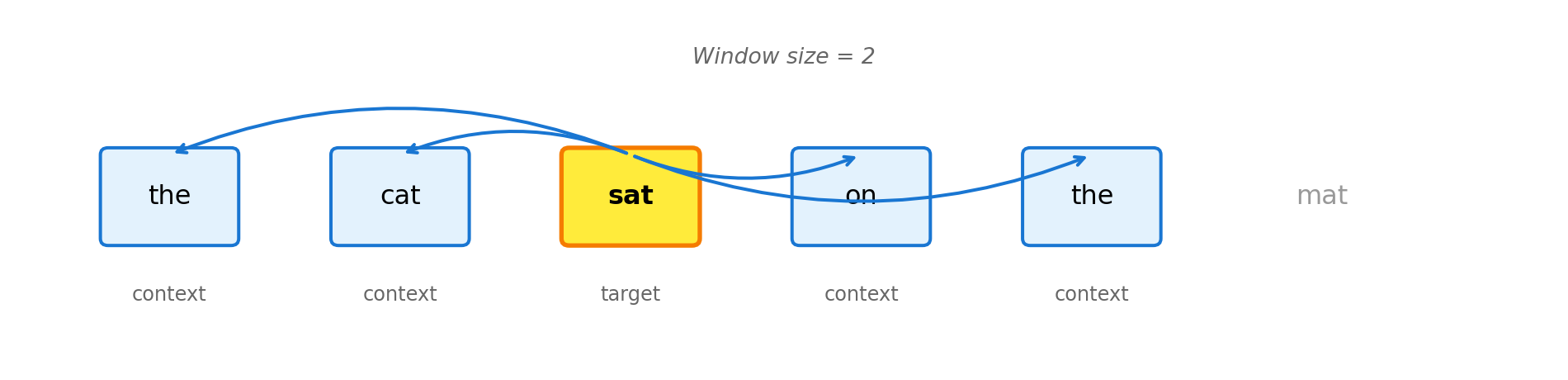
Figure 4.3: Skip-gram: given a target word, predict context words within a window. Here, ‘sat’ predicts ‘the’, ‘cat’, ‘on’, ‘the’.
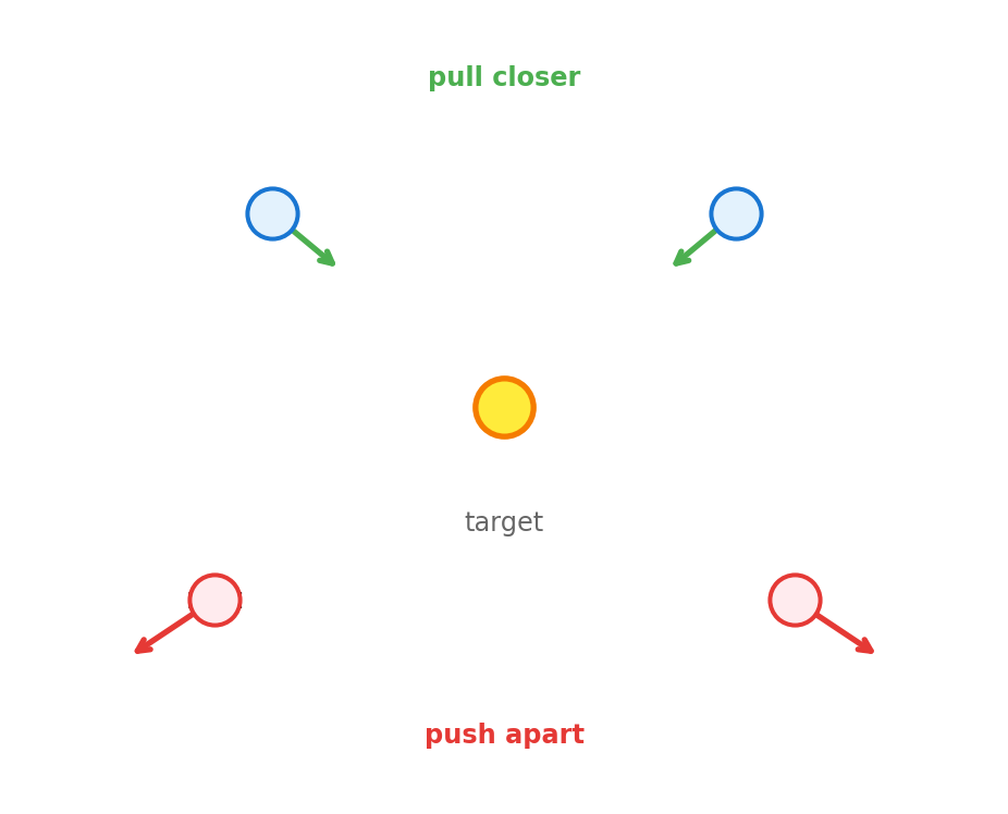
The implementation below shows the core training loop: for each target-context pair from real text, push their embeddings closer together; for random “negative” pairs, push them apart. After enough iterations, similar words cluster in embedding space.
Figure 4.4: Training pushes context words closer to target (green arrows) and negative samples farther away (red arrows).
"""Word2Vec Skip-Gram: Simplified Implementation"""import numpy as np# Training data: sentences we learn word relationships fromcorpus = [["the", "cat", "sat", "on", "the", "mat"], ["the", "dog", "sat", "on", "the", "rug"]]# Vocabulary: unique words extracted from corpusvocab =list(set(word for sentence in corpus for word in sentence))vocab_size =len(vocab)embedding_dim =4# Small for demo; production uses 100-300 dimensionsword_to_idx = {w: i for i, w inenumerate(vocab)}# Initialize two embedding matrices with small random valuesnp.random.seed(42)W_target = np.random.randn(vocab_size, embedding_dim) *0.1W_context = np.random.randn(vocab_size, embedding_dim) *0.1def sigmoid(x):"""Squash any value to range (0, 1). Clip prevents overflow."""return1/ (1+ np.exp(-np.clip(x, -500, 500)))def train_skipgram_pair(target_word, context_word, negative_words, lr=0.1):"""Train on one (target, context) pair with negative sampling. Example: in "the cat sat", target="cat", context="the" or "sat", negatives=["dog", "rug"] (random words not in context). """global W_target, W_context t_idx = word_to_idx[target_word] c_idx = word_to_idx[context_word] target_emb = W_target[t_idx] context_emb = W_context[c_idx]# Positive example: target and context should be similar score = np.dot(target_emb, context_emb) pred = sigmoid(score) W_target[t_idx] -= lr * (pred -1) * context_emb W_context[c_idx] -= lr * (pred -1) * target_emb# Negative examples: push apart words that don't appear together.# Without this, model would collapse all embeddings to the same point.for neg_word in negative_words: n_idx = word_to_idx[neg_word] neg_emb = W_context[n_idx] score = np.dot(target_emb, neg_emb) pred = sigmoid(score) W_target[t_idx] -= lr * pred * neg_emb W_context[n_idx] -= lr * pred * target_emb# Each epoch = one pass through corpus. Multiple passes needed because# each example only nudges embeddings slightly; repetition reinforces patterns.for epoch inrange(50):for sentence in corpus:for i, target inenumerate(sentence):# Context = words within 2 positions of target start =max(0, i -2) end =min(len(sentence), i +3) context_words = [sentence[j] for j inrange(start, end) if j != i]# Negatives = random words not appearing near target negatives = [w for w in vocab if w notin context_words and w != target][:2]for context in context_words: train_skipgram_pair(target, context, negatives)# cosine_similarity = (A · B) / (||A|| × ||B||)def cosine_similarity(w1, w2): v1, v2 = W_target[word_to_idx[w1]], W_target[word_to_idx[w2]]return np.dot(v1, v2) / (np.linalg.norm(v1) * np.linalg.norm(v2))print("Learned similarities:")print(f" cat ↔ dog: {cosine_similarity('cat', 'dog'):.3f}")print(f" cat ↔ mat: {cosine_similarity('cat', 'mat'):.3f}")
Why is cat↔︎mat higher than cat↔︎dog? In our tiny corpus, “cat” and “mat” appear in the same sentence, sharing more context words. Word2Vec learns from co-occurrence patterns in the training data—with millions of sentences, “cat” and “dog” would cluster together as animals, but our two-sentence corpus doesn’t capture that relationship.
4.7.2 BERT: Contextual Token Embeddings
The transformer architecture (Vaswani et al. 2017) and BERT (Devlin et al. 2018) introduced contextual embeddings—the same word gets different representations based on context.
The key innovation is the attention mechanism: when processing a word, the model can “look at” all other words in the sentence to determine meaning. This is fundamentally different from Word2Vec:
Word2Vec: Context matters during training (learning from nearby words), but produces static embeddings. Once trained, “bank” always maps to the same vector—the model can’t tell which meaning you intend.
Transformers: Context matters at inference time. Each time you encode a sentence, the model examines all surrounding words to compute a contextual embedding. “Bank” gets different vectors depending on whether the sentence mentions money or rivers.
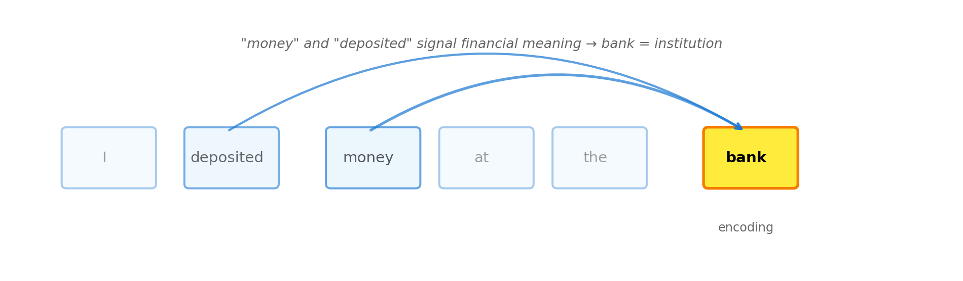
Figure 4.5: Attention mechanism: when encoding ‘bank’, the model attends to other words to determine meaning. ‘Money’ and ‘deposited’ signal financial meaning.
Unlike Word2Vec (where we showed training from scratch), we won’t implement transformer training here. Why? Scale. Word2Vec trains in minutes on a laptop with a few sentences. BERT was trained on 3.3 billion words using 64 TPUs for 4 days. The architecture is also far more complex—multi-head attention, layer normalization, positional encodings, and masked language modeling objectives.
Instead, we use pre-trained models. The code below loads a model that’s already learned contextual representations from massive text corpora:
"""Contextual Embeddings: Same Word, Different Meanings"""from sentence_transformers import SentenceTransformerfrom sklearn.metrics.pairwise import cosine_similarity# Load pre-trained transformer modelmodel = SentenceTransformer('all-MiniLM-L6-v2')# Same word "bank" in different contextssentences = ["I deposited money at the bank", # financial-1"The bank approved my loan", # financial-2"We had a picnic on the river bank", # river-1"Fish swim near the bank", # river-2]# Each sentence gets a single embedding capturing its full meaningembeddings = model.encode(sentences)print("Sentence similarity (same meaning = higher score):\n")labels = ["financial-1", "financial-2", "river-1", "river-2"]for i inrange(len(sentences)):for j inrange(i +1, len(sentences)): sim = cosine_similarity([embeddings[i]], [embeddings[j]])[0][0]print(f" {labels[i]:12s} ↔ {labels[j]:12s}: {sim:.3f}")
The financial sentences (0.486) are more similar to each other than to river sentences, and vice versa—but the differences aren’t dramatic. Is this a limitation? It depends on your use case:
For sentence-level tasks (semantic search, document clustering), this is fine. The embeddings correctly distinguish the sentence meanings, just not by a huge margin.
For word-sense disambiguation (detecting that “bank” means different things), you need token-level embeddings instead of sentence embeddings. BERT produces distinct embeddings for “bank” in each context—the pooling step that creates a single sentence embedding averages this information away.
To get the contextual embedding for a specific word, use the underlying BERT model directly and extract the token’s hidden state, rather than using a Sentence Transformer that pools all tokens together.
Why transformers dominate:
Parallelization: All words processed simultaneously. Earlier models (RNNs—Recurrent Neural Networks) processed words one at a time, left to right. This was slow and made training on large datasets impractical.
Long-range dependencies: Attention connects distant words directly. In “The cat that I saw yesterday at the park was sleeping”, attention links “cat” to “sleeping” without processing all words in between.
Transfer learning: Pre-trained models work across many tasks without retraining from scratch.
Scalability: Performance improves predictably with more data and compute.
The previous section covered BERT—a powerful architecture that produces token-level embeddings. But throughout this chapter, we’ve been using SentenceTransformer to get sentence-level embeddings. What’s the connection?
Sentence Transformers (Reimers and Gurevych 2019) are BERT models fine-tuned specifically for producing useful sentence embeddings. The problem: raw BERT produces one embedding per token, not per sentence. The naive fix—averaging all token embeddings—works poorly because it weights filler words (“the”, “a”) equally with meaningful ones.
Sentence Transformers solve this using a siamese architecture: two identical BERT models process two sentences, then a pooling layer (typically mean or [CLS] token) produces one embedding each. Training uses contrastive learning—the model learns to produce similar embeddings for related sentences (paraphrases, question-answer pairs) and dissimilar embeddings for unrelated ones.
TipKey Resources
Sentence-BERT paper (Reimers & Gurevych, 2019) — the original Sentence Transformers paper
Figure 4.6: Sentence Transformer training: a siamese network processes sentence pairs through identical BERT encoders. Paraphrases are pushed together; unrelated sentences are pushed apart.
The key insight: by training on millions of sentence pairs (from datasets like NLI, paraphrase corpora, and question-answer pairs), the model learns to capture semantic similarity—not just surface-level word overlap. This is why Sentence Transformers produce excellent embeddings out of the box, unlike raw BERT which needs task-specific fine-tuning.
For a deeper dive into contrastive learning techniques, see Chapter 15. For training your own sentence embeddings, see Chapter 14.
4.8 Key Takeaways
Text embeddings convert words, sentences, or documents into vectors capturing semantic meaning
Similar text → similar vectors: This enables semantic search, clustering, and classification without explicit rules
Popular models range from fast (MiniLM) to high-quality (OpenAI text-embedding-3) depending on your needs
Word2Vec learns from word co-occurrence patterns—words in similar contexts get similar embeddings
Transformers (BERT) create contextual embeddings where the same word gets different vectors based on surrounding context
Sentence Transformers adapt these for producing single embeddings for entire sentences
4.9 Looking Ahead
Now that you understand text embeddings, Chapter 5 explores how similar principles apply to visual data—images and video.
4.10 Further Reading
Mikolov, T., et al. (2013). “Efficient Estimation of Word Representations in Vector Space.” arXiv:1301.3781
Vaswani, A., et al. (2017). “Attention Is All You Need.” NeurIPS
Devlin, J., et al. (2018). “BERT: Pre-training of Deep Bidirectional Transformers.” arXiv:1810.04805
Reimers, N. & Gurevych, I. (2019). “Sentence-BERT: Sentence Embeddings using Siamese BERT-Networks.” arXiv:1908.10084
Devlin, Jacob, Ming-Wei Chang, Kenton Lee, and Kristina Toutanova. 2018. “BERT: Pre-Training of Deep Bidirectional Transformers for Language Understanding.”arXiv Preprint arXiv:1810.04805.
Mikolov, Tomas, Kai Chen, Greg Corrado, and Jeffrey Dean. 2013. “Efficient Estimation of Word Representations in Vector Space.”arXiv Preprint arXiv:1301.3781.
Reimers, Nils, and Iryna Gurevych. 2019. “Sentence-BERT: Sentence Embeddings Using Siamese BERT-Networks.”arXiv Preprint arXiv:1908.10084.
Vaswani, Ashish, Noam Shazeer, Niki Parmar, Jakob Uszkoreit, Llion Jones, Aidan N Gomez, Lukasz Kaiser, and Illia Polosukhin. 2017. “Attention Is All You Need.”Advances in Neural Information Processing Systems 30.