5 Image, Audio, and Video Embeddings
NoteChapter Overview
This chapter covers embeddings for visual and audio data—images, audio, and video. We explore how these modalities are represented as vectors, when to use each type, and the architectures that create them. An optional advanced section explains how the underlying models learn visual features.
5.1 Image Embeddings
Image embeddings convert visual content into vectors that capture visual semantics—shapes, colors, textures, objects, and spatial relationships. Unlike pixel-by-pixel comparison, embeddings understand that two photos of the same cat are similar even if taken from different angles or lighting conditions.
The example below uses ResNet50 (He et al. 2016), a CNN pre-trained on ImageNet’s 1.4 million images. ResNet learns hierarchical visual features—early layers detect edges and textures, middle layers recognize shapes and parts, and deep layers understand objects and scenes. We remove the final classification layer to extract the 2048-dimensional feature vector as our embedding.
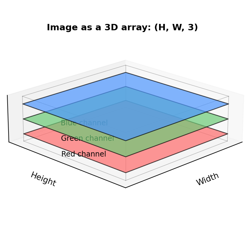
Digital images are stored as 3D arrays with shape (height, width, 3)—the third dimension holds Red, Green, and Blue color intensities for each pixel:
"""
Image Embeddings: Visual Content as Vectors
"""

import torch
import numpy as np
from PIL import Image
from torchvision import models, transforms
from sklearn.metrics.pairwise import cosine_similarity

# Suppress download messages
import logging
logging.getLogger('torch').setLevel(logging.ERROR)

from torchvision.models import ResNet50_Weights

# Load pretrained ResNet50 as feature extractor
weights = ResNet50_Weights.IMAGENET1K_V1
model = models.resnet50(weights=None)
model.load_state_dict(weights.get_state_dict(progress=False))
model.eval()

# Remove classification head to get embeddings
feature_extractor = torch.nn.Sequential(*list(model.children())[:-1])

# Standard ImageNet preprocessing
preprocess = transforms.Compose([
    transforms.Resize(256),
    transforms.CenterCrop(224),
    transforms.ToTensor(),
    transforms.Normalize(mean=[0.485, 0.456, 0.406], std=[0.229, 0.224, 0.225]),
])

def get_image_embedding(image):
    """Extract embedding from PIL Image."""
    tensor = preprocess(image).unsqueeze(0)
    with torch.no_grad():
        embedding = feature_extractor(tensor)
    return embedding.squeeze().numpy()

# Create synthetic test images with different color patterns
# np.random.randint([low_r, low_g, low_b], [high_r, high_g, high_b], shape)
# generates random RGB values within the specified range for each pixel
np.random.seed(42)
images = {
    'red_pattern': Image.fromarray(
        np.random.randint([180, 0, 0], [255, 80, 80], (224, 224, 3), dtype=np.uint8)
    ),
    'blue_pattern': Image.fromarray(
        np.random.randint([0, 0, 180], [80, 80, 255], (224, 224, 3), dtype=np.uint8)
    ),
    'orange_pattern': Image.fromarray(
        np.random.randint([200, 100, 0], [255, 150, 50], (224, 224, 3), dtype=np.uint8)
    ),
}

# Get embeddings
embeddings = {name: get_image_embedding(img) for name, img in images.items()}

print("Image embedding similarities:\n")
print("Red and orange (similar warm colors) should be more similar than red and blue:")
red_orange = cosine_similarity([embeddings['red_pattern']], [embeddings['orange_pattern']])[0][0]
red_blue = cosine_similarity([embeddings['red_pattern']], [embeddings['blue_pattern']])[0][0]
print(f"  red ↔ orange: {red_orange:.3f}")
print(f"  red ↔ blue:   {red_blue:.3f}")
Image embedding similarities:
Red and orange (similar warm colors) should be more similar than red and blue:
red ↔ orange: 0.898
red ↔ blue: 0.717Show RGB channel visualization code
import matplotlib.pyplot as plt
import matplotlib.gridspec as gridspec

fig = plt.figure(figsize=(12, 4))
gs = gridspec.GridSpec(3, 7, width_ratios=[3, 0.5, 3, 0.5, 3, 0.5, 3], hspace=0.1, wspace=0.05)

for row, (name, img) in enumerate(images.items()):
    img_array = np.array(img)
    label = name.replace("_pattern", "").title()

    ax = fig.add_subplot(gs[row, 0])
    ax.imshow(img)
    if row == 0:
        ax.set_title(label, fontsize=10)
    ax.axis('off')

    ax = fig.add_subplot(gs[row, 1])
    ax.text(0.5, 0.5, '=', fontsize=16, ha='center', va='center', fontweight='bold')
    ax.axis('off')

    ax = fig.add_subplot(gs[row, 2])
    ax.imshow(img_array[:,:,0], cmap='Reds', vmin=0, vmax=255)
    if row == 0:
        ax.set_title('R', fontsize=10)
    ax.axis('off')

    ax = fig.add_subplot(gs[row, 3])
    ax.text(0.5, 0.5, '+', fontsize=16, ha='center', va='center', fontweight='bold')
    ax.axis('off')

    ax = fig.add_subplot(gs[row, 4])
    ax.imshow(img_array[:,:,1], cmap='Greens', vmin=0, vmax=255)
    if row == 0:
        ax.set_title('G', fontsize=10)
    ax.axis('off')

    ax = fig.add_subplot(gs[row, 5])
    ax.text(0.5, 0.5, '+', fontsize=16, ha='center', va='center', fontweight='bold')
    ax.axis('off')

    ax = fig.add_subplot(gs[row, 6])
    ax.imshow(img_array[:,:,2], cmap='Blues', vmin=0, vmax=255)
    if row == 0:
        ax.set_title('B', fontsize=10)
    ax.axis('off')

plt.suptitle('RGB: Three 2D channels combine to create color images', fontsize=11, fontweight='bold', y=0.98)
plt.show()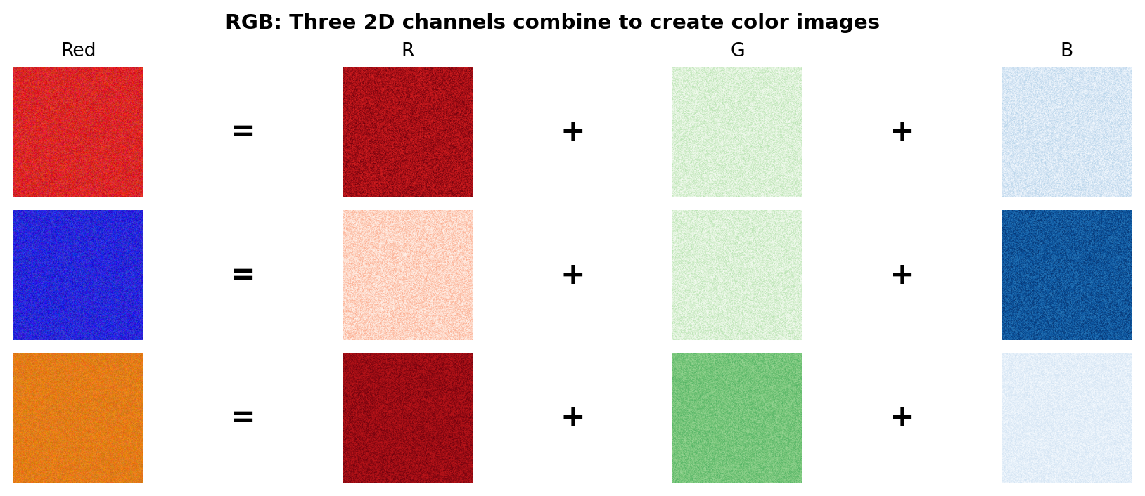
When comparing image embeddings, we use cosine similarity just like with text. Images with similar visual features—colors, textures, shapes, or objects—will have embeddings that point in similar directions, yielding high similarity scores. The red and orange patterns share warm color features, so their embeddings are closer together than red and blue. In practice, this means a photo of a red dress will be more similar to an orange dress than a blue one, even though all three are “dresses.”
How does the model “understand” colors? As Figure 5.2 shows, each image is stored as three 2D arrays—one for Red, Green, and Blue intensity. The red pattern has high values in the R channel and low values in G and B. Orange combines high R with medium G (red + green = orange).
NoteRGB Input ≠ Embedding Output
Don’t confuse the 3-channel RGB input with the embedding output. ResNet50 takes the 3 RGB channels as input but produces a 2048-dimensional embedding vector that captures far more than color: edges, textures, shapes, and high-level visual concepts learned from millions of images.
The model receives the three RGB channels as input, and early CNN layers learn filters that activate for specific patterns—some respond to warm tones, others to edges or textures. As layers get deeper, the network combines these low-level features into increasingly abstract representations. By training on millions of labeled images, the model learns that red and orange often appear together (sunsets, autumn leaves, fire) more frequently than red and blue, encoding this statistical relationship across all 2048 dimensions.
Beyond colors, early CNN layers also learn edge detectors—filters that respond to boundaries between light and dark regions. For a hands-on introduction to how a single neuron learns to detect edges, see How Neural Networks Learn to See.
When to use image embeddings:
- Visual recommendation systems—suggest visually similar items (see Chapter 13)
- Content moderation—detect variations of prohibited images (see Section 26.7)
- Forensic video search—find specific people or objects in footage (see Chapter 27) (reverse image lookup)
- Face recognition—identify or verify individuals from photos (see Chapter 27)
- Duplicate and near-duplicate detection—identify copied or modified images (see Chapter 28) (reverse image lookup)
- Medical imaging—find similar X-rays, scans, or pathology slides (see Chapter 30)
- Visual product search—find products similar to a photo (see Chapter 31) (reverse image lookup)
- Quality control—detect defects by comparing to reference images (see Chapter 32)
There are dozens of other applications including art style matching, stock photo search, image classification, trademark and logo detection, scene recognition, wildlife identification, satellite imagery analysis, document scanning, and autonomous vehicle perception.
Popular architectures:
| Architecture | Type | Strengths | Use Cases |
|---|---|---|---|
| ResNet | CNN | Fast, proven | General visual search |
| EfficientNet | CNN | Efficient, accurate | Mobile/edge deployment |
| ViT | Transformer | Best accuracy | High-quality requirements |
| CLIP | Multi-modal | Text-image alignment | Zero-shot classification |
5.2 Audio Embeddings
Audio embeddings convert sound into vectors that capture acoustic properties—pitch, timbre, rhythm, and spectral characteristics. Unlike raw waveform comparison, embeddings understand that two recordings of the same spoken word are similar even with different speakers, background noise, or recording equipment.
The example below uses MFCC (Mel-frequency cepstral coefficients), a classic signal processing technique—not a neural network, but a fixed mathematical transformation that extracts acoustic features. MFCCs transform audio into a representation that mimics human hearing—emphasizing frequencies we’re sensitive to while compressing less important details. While modern systems use learned embeddings from models like Wav2Vec2, MFCCs remain useful as a baseline and for understanding what acoustic features matter.
We extract 20 values per time frame, called coefficients—each describes a different aspect of the sound’s frequency content (overall loudness, balance between low and high frequencies, etc.). Since audio clips vary in length (a 3-second clip has more frames than a 1-second clip), we aggregate across time using mean and standard deviation to create a fixed-size embedding that works regardless of duration:

"""
Audio Embeddings: Sound as Vectors
"""

import numpy as np
import librosa
from sklearn.metrics.pairwise import cosine_similarity

def audio_to_embedding(audio, sr, n_mfcc=20):
    """Convert audio waveform to a fixed-size embedding using MFCCs."""
    # Extract MFCCs: 20 coefficients per time frame
    mfccs = librosa.feature.mfcc(y=audio, sr=sr, n_mfcc=n_mfcc)
    # Aggregate over time: mean captures average timbre, std captures variation
    return np.concatenate([mfccs.mean(axis=1), mfccs.std(axis=1)])

# Load librosa's built-in trumpet sample
audio, sr = librosa.load(librosa.ex('trumpet'))
trumpet_embedding = audio_to_embedding(audio, sr)

# Create variations to demonstrate similarity
trumpet_slow = librosa.effects.time_stretch(audio, rate=0.8)
trumpet_pitch_up = librosa.effects.pitch_shift(audio, sr=sr, n_steps=12)  # One octave up

# Generate embeddings for each variation
embeddings = {
    'trumpet_original': trumpet_embedding,
    'trumpet_slower': audio_to_embedding(trumpet_slow, sr),
    'trumpet_higher_pitch': audio_to_embedding(trumpet_pitch_up, sr),
}

print(f"Embedding dimension: {len(trumpet_embedding)} (20 MFCCs × 2 stats)\n")

# Compare similarities
print("Audio embedding similarities:")
sim_slow = cosine_similarity(
    [embeddings['trumpet_original']], [embeddings['trumpet_slower']]
)[0][0]
print(f"  Original ↔ Slower tempo:   {sim_slow:.3f}")

sim_pitch = cosine_similarity(
    [embeddings['trumpet_original']], [embeddings['trumpet_higher_pitch']]
)[0][0]
print(f"  Original ↔ Higher pitch:   {sim_pitch:.3f}")

sim_variations = cosine_similarity(
    [embeddings['trumpet_slower']], [embeddings['trumpet_higher_pitch']]
)[0][0]
print(f"  Slower ↔ Higher pitch:     {sim_variations:.3f}")
Embedding dimension: 40 (20 MFCCs × 2 stats)
Audio embedding similarities:
Original ↔ Slower tempo: 1.000
Original ↔ Higher pitch: 0.978
Slower ↔ Higher pitch: 0.980When comparing audio embeddings, cosine similarity measures how acoustically similar two sounds are. Notice that all similarities are high (>0.97)—this is by design. MFCCs capture timbre (the trumpet’s characteristic “brassy” quality) rather than absolute pitch or tempo. The tempo change preserves timbre almost perfectly (1.000), while shifting pitch by an octave causes only a small drop (~0.98) because the overall spectral shape remains trumpet-like. This robustness is useful for applications like speaker identification, where you want to match voices regardless of speaking speed or emotional pitch variations.
How do MFCCs capture sound? Audio is first split into short overlapping frames (typically 25ms). For each frame, we compute the frequency spectrum, then apply a mel filterbank that groups frequencies into bands matching human perception—more resolution at low frequencies where we hear pitch differences, less at high frequencies. The cepstral coefficients compress this further, capturing the overall “shape” of the spectrum. The result: a compact representation of timbre that’s robust to volume changes.
When to use audio embeddings: Content moderation, audio fingerprinting, speaker identification, music recommendation, podcast and video search, sound event detection, voice cloning detection, acoustic quality control, wildlife monitoring, and medical diagnostics from sounds (coughs, heartbeats).
This book covers music recommendation with audio embeddings in Chapter 13. If you’d like to see other audio applications covered in future editions, reach out to the author.
Popular architectures:
| Architecture | Type | Strengths | Use Cases |
|---|---|---|---|
| Wav2Vec2 | Self-supervised | Rich speech features | Speech recognition, speaker ID |
| Whisper | Multi-task | Transcription + embeddings | Speech search, subtitles |
| CLAP | Multi-modal | Audio-text alignment | Zero-shot audio classification |
| VGGish | CNN | General audio events | Sound classification |
For audio model architecture details, see the linked documentation above or explore the Hugging Face Audio Course for a comprehensive introduction.
5.3 Video Embeddings
Video embeddings convert video clips into vectors that capture both visual content and temporal dynamics—actions, motion patterns, scene transitions, and narrative flow. Unlike image embeddings that capture a single moment, video embeddings understand that “a person sitting down” and “a person standing up” are different actions even though individual frames might look similar.
The challenge with video is combining spatial information (what’s in each frame) with temporal information (how things change over time). The simplest approach extracts image embeddings from sampled frames and aggregates them. More sophisticated models process multiple frames together to capture motion directly.
Just as images are 3D arrays (height × width × 3 channels), videos add a fourth dimension: time. A video is a sequence of frames, each of which is an image:
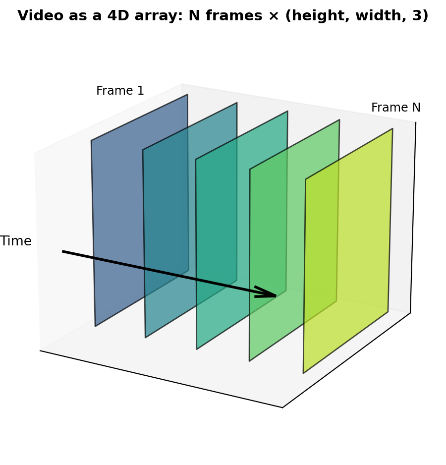
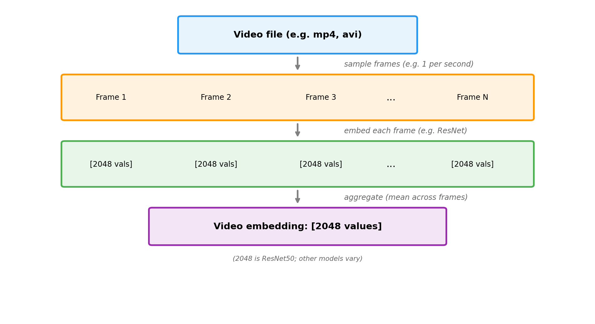
The example below demonstrates the frame sampling approach: we extract image embeddings from frames sampled throughout a video, then average them to create a single video embedding. Since videos vary in length, aggregation (like we saw with audio) produces a fixed-size embedding regardless of duration.
"""
Video Embeddings: From Clips to Vectors
"""

import torch
import numpy as np
from torchvision import models, transforms
from torchvision.models import ResNet50_Weights
from sklearn.metrics.pairwise import cosine_similarity

# Suppress download messages
import logging
logging.getLogger('torch').setLevel(logging.ERROR)

# Load pretrained ResNet50 as frame feature extractor
weights = ResNet50_Weights.IMAGENET1K_V1
model = models.resnet50(weights=None)
model.load_state_dict(weights.get_state_dict(progress=False))
model.eval()
feature_extractor = torch.nn.Sequential(*list(model.children())[:-1])

# Normalize using ImageNet statistics: the mean and std of RGB values across
# 1.2M training images. This ensures our input has the same distribution the
# model was trained on. These specific values are standard for ImageNet models.
preprocess = transforms.Compose([
    transforms.ToTensor(),
    transforms.Normalize(mean=[0.485, 0.456, 0.406], std=[0.229, 0.224, 0.225]),
])

def frames_to_video_embedding(frames):
    """Convert a list of frames (as numpy arrays) to a video embedding."""
    frame_embeddings = []
    for frame in frames:
        # Convert numpy array to tensor and preprocess
        if frame.dtype == np.uint8:
            frame = frame.astype(np.float32) / 255.0
        tensor = preprocess(frame).unsqueeze(0)
        with torch.no_grad():
            emb = feature_extractor(tensor).squeeze().numpy()
        frame_embeddings.append(emb)
    # Aggregate: mean across all frames
    return np.mean(frame_embeddings, axis=0)

# Simulate video frames as colored images (224x224 RGB)
# "Running video": frames transition from green (grass) to blue (sky) - outdoor motion
running_frames = [
    np.full((224, 224, 3), [0.2, 0.6 + i*0.05, 0.2], dtype=np.float32)  # Green to lighter
    for i in range(5)
]

# "Cooking video": frames stay warm orange/red tones - kitchen scene
cooking_frames = [
    np.full((224, 224, 3), [0.8, 0.4 + i*0.02, 0.1], dtype=np.float32)  # Warm tones
    for i in range(5)
]

# "Jogging video": similar to running - outdoor greens and blues
jogging_frames = [
    np.full((224, 224, 3), [0.25, 0.55 + i*0.05, 0.25], dtype=np.float32)  # Similar greens
    for i in range(5)
]

# Generate video embeddings
embeddings = {
    'running': frames_to_video_embedding(running_frames),
    'cooking': frames_to_video_embedding(cooking_frames),
    'jogging': frames_to_video_embedding(jogging_frames),
}

print(f"Video embedding dimension: {len(embeddings['running'])}\n")
print("Video embedding similarities:")

run_jog = cosine_similarity([embeddings['running']], [embeddings['jogging']])[0][0]
run_cook = cosine_similarity([embeddings['running']], [embeddings['cooking']])[0][0]
jog_cook = cosine_similarity([embeddings['jogging']], [embeddings['cooking']])[0][0]

print(f"  Running ↔ Jogging: {run_jog:.3f}  (similar outdoor scenes)")
print(f"  Running ↔ Cooking: {run_cook:.3f}  (different scenes)")
print(f"  Jogging ↔ Cooking: {jog_cook:.3f}  (different scenes)")
Video embedding dimension: 2048
Video embedding similarities:
Running ↔ Jogging: 0.995 (similar outdoor scenes)
Running ↔ Cooking: 0.807 (different scenes)
Jogging ↔ Cooking: 0.808 (different scenes)Show video frame visualization code
import matplotlib.pyplot as plt
import matplotlib.gridspec as gridspec

fig = plt.figure(figsize=(12, 4))
gs = gridspec.GridSpec(3, 7, width_ratios=[3, 0.3, 3, 0.3, 3, 0.3, 3], hspace=0.15, wspace=0.05)

videos = [
    ('Running', running_frames),
    ('Cooking', cooking_frames),
    ('Jogging', jogging_frames),
]

for row, (name, frames) in enumerate(videos):
    # Show 4 sample frames from the video
    frame_indices = [0, 1, 3, 4]  # Sample frames

    for col, fidx in enumerate(frame_indices):
        ax = fig.add_subplot(gs[row, col * 2])
        ax.imshow(frames[fidx])
        if row == 0:
            ax.set_title(f'Frame {fidx + 1}', fontsize=9)
        ax.set_xticks([])
        ax.set_yticks([])
        for spine in ax.spines.values():
            spine.set_visible(False)

        # Add video name label on left side of first frame
        if col == 0:
            ax.text(-0.15, 0.5, name, fontsize=10, fontweight='bold',
                    transform=ax.transAxes, ha='right', va='center')

        # Add arrow between frames (except last)
        if col < 3:
            ax_arrow = fig.add_subplot(gs[row, col * 2 + 1])
            ax_arrow.text(0.5, 0.5, '→', fontsize=14, ha='center', va='center', color='gray')
            ax_arrow.axis('off')

plt.suptitle('Video frames: similar scenes have similar color patterns across time', fontsize=11, fontweight='bold', y=0.98)
plt.show()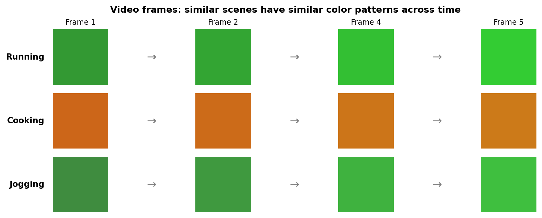
When comparing video embeddings, similar activities and scenes cluster together. Running and jogging videos both contain outdoor scenes with similar color palettes (greens, blues), so their embeddings are close. Cooking videos have warm indoor tones (oranges, reds) that differ significantly from outdoor activities.
The frame sampling approach shown above is simple but misses motion information—it can’t distinguish “sitting down” from “standing up” since both might have similar individual frames. More advanced architectures like SlowFast and Video Swin (see table below) process multiple frames together using 3D convolutions or temporal attention, capturing how pixels change over time to understand motion and actions.
When to use video embeddings: Action recognition and search, video recommendation, content moderation, surveillance and anomaly detection, video summarization, sports analytics, and gesture recognition.
This book covers video surveillance applications in Chapter 27. If you’d like to see other video applications covered in future editions, reach out to the author.
Popular architectures:
| Architecture | Type | Strengths | Use Cases |
|---|---|---|---|
| Frame sampling + CNN | Aggregated image embeddings | Simple, fast (no motion) | Scene classification |
| SlowFast | Two-pathway 3D CNN | Captures fast and slow motion | Action recognition |
| X3D | Efficient 3D CNN | Mobile-friendly | Real-time applications |
| Video Swin | Video transformer | State-of-the-art accuracy | High-quality requirements |
For video model architecture details, see the linked documentation above.
5.4 Advanced: How Visual Models Learn
NoteOptional Section
This section explains how image embedding models learn visual features. Understanding these fundamentals helps you choose the right model and fine-tune for your domain. Skip this if you just need to use embeddings.
5.4.1 Convolutional Neural Networks (CNNs)
CNNs learn hierarchical visual features through layers of convolution operations:
- Early layers detect edges and textures—horizontal lines, vertical lines, gradients
- Middle layers combine edges into shapes—corners, curves, patterns
- Deep layers recognize objects—faces, cars, animals
Each convolutional filter acts as a pattern detector, sliding across the image and activating when it finds its learned pattern. Through training on millions of labeled images, these filters learn increasingly abstract representations.
5.4.2 Vision Transformers (ViT)
Vision Transformers apply the same attention mechanism from text to images by:
- Splitting the image into patches (e.g., 16×16 pixels each)
- Treating each patch as a “token” (like words in text)
- Applying transformer layers to learn relationships between patches
This allows ViT to capture long-range dependencies—understanding that distant parts of an image are related—which CNNs struggle with due to their local receptive fields.
5.4.3 Transfer Learning
Most applications don’t train image models from scratch. Instead:
- Start with a model pre-trained on ImageNet (1.4M labeled images)
- Remove the classification head to get feature vectors
- Optionally fine-tune on your domain-specific data
This works because low-level features (edges, textures) transfer across domains—a model that learned to detect edges on ImageNet can detect edges in medical images or satellite photos.
5.5 Key Takeaways
- Image embeddings capture visual semantics—similar objects, colors, and textures cluster together regardless of exact pixel values
- Audio embeddings capture acoustic properties—timbre, rhythm, and spectral features that identify sounds across variations
- Video embeddings combine spatial and temporal information—understanding both what’s in each frame and how things change over time
- CNNs learn hierarchical features through convolution layers; Vision Transformers use attention to capture long-range relationships
- Transfer learning is standard practice—start with pre-trained models and adapt to your domain
5.6 Looking Ahead
Now that you understand single-modality embeddings for text, images, audio, and video, Chapter 6 explores how to combine these modalities into unified multi-modal representations.
5.7 Further Reading
- He, K., et al. (2016). “Deep Residual Learning for Image Recognition.” CVPR
- Dosovitskiy, A., et al. (2020). “An Image is Worth 16x16 Words: Transformers for Image Recognition at Scale.” ICLR
- Gemmeke, J., et al. (2017). “Audio Set: An ontology and human-labeled dataset for audio events.” ICASSP
- Feichtenhofer, C., et al. (2019). “SlowFast Networks for Video Recognition.” ICCV