8  Time-Series Embeddings

NoteChapter Overview

This chapter covers time-series embeddings—representations that convert sequences of measurements over time into vectors capturing temporal patterns. We explore how these embeddings detect trends, seasonality, cycles, and anomalies, enabling applications from predictive maintenance to financial pattern recognition.

8.1 What Are Time-Series Embeddings?

Time-series embeddings convert sequences of measurements over time into vectors that capture temporal patterns—trends, seasonality, cycles, and anomalies. Two sensors with similar behavior patterns (e.g., both showing daily cycles) will have similar embeddings, even if their absolute values differ.

The challenge: patterns exist at multiple scales—short-term fluctuations, medium-term trends, and long-term seasonality. Like audio, time-series vary in length, so embeddings must aggregate temporal information into fixed-size vectors.

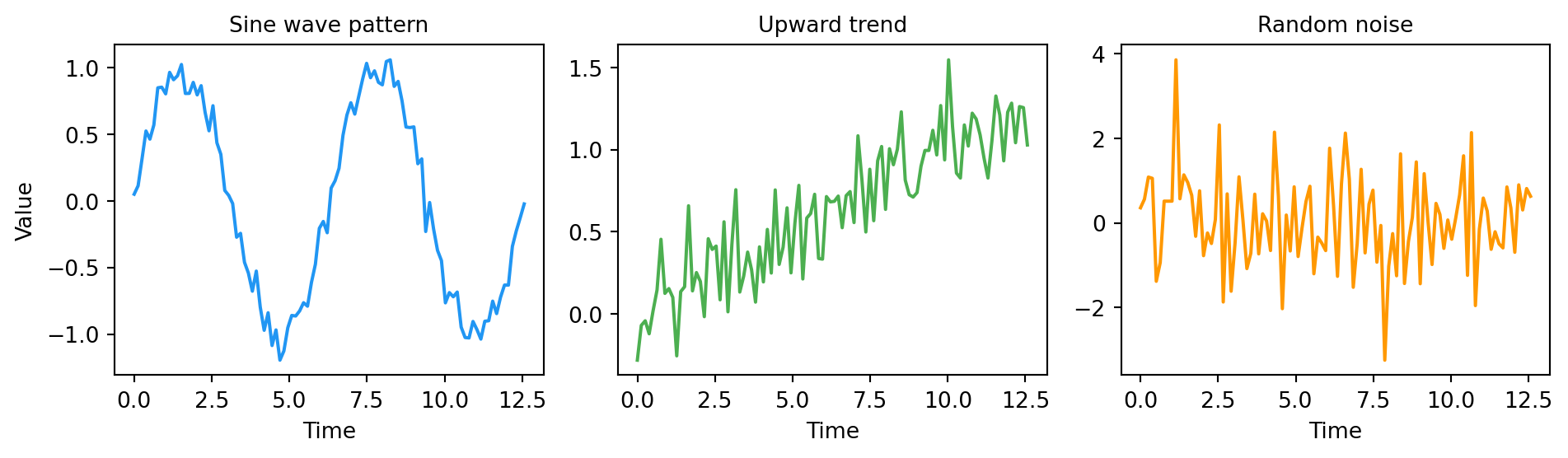
8.2 Visualizing Time-Series Patterns

Figure 8.1: Time-series patterns: sine waves and upward trends have distinct signatures that embeddings capture.

8.3 Creating Time-Series Embeddings

"""
Time-Series Embeddings: Temporal Patterns as Vectors
"""

import numpy as np
from sklearn.metrics.pairwise import cosine_similarity

np.random.seed(42)

def generate_pattern(pattern_type, length=100):
    """Generate synthetic time-series with specific patterns."""
    t = np.linspace(0, 4*np.pi, length)
    if pattern_type == 'sine':
        return np.sin(t) + np.random.randn(length) * 0.1
    elif pattern_type == 'increasing':
        return t/10 + np.random.randn(length) * 0.2
    else:
        return np.random.randn(length)

def timeseries_embedding(series):
    """Extract statistical features as a simple embedding."""
    return np.array([
        np.mean(series),                              # level
        np.std(series),                               # variability
        np.max(series) - np.min(series),              # range
        np.mean(np.diff(series)),                     # trend (avg change)
        np.corrcoef(series[:-1], series[1:])[0, 1],   # autocorrelation
    ])

# Generate time-series with different patterns
patterns = {
    'sine_wave_1': generate_pattern('sine'),
    'sine_wave_2': generate_pattern('sine'),
    'trend_up_1': generate_pattern('increasing'),
    'trend_up_2': generate_pattern('increasing'),
}

embeddings = {name: timeseries_embedding(ts) for name, ts in patterns.items()}

print(f"Embedding dimension: {len(embeddings['sine_wave_1'])} (5 statistical features)\n")
print("Time-series embedding similarities:\n")
print("Same pattern type:")
sine_sim = cosine_similarity([embeddings['sine_wave_1']], [embeddings['sine_wave_2']])[0][0]
trend_sim = cosine_similarity([embeddings['trend_up_1']], [embeddings['trend_up_2']])[0][0]
print(f"  Sine wave 1 ↔ Sine wave 2: {sine_sim:.3f}")
print(f"  Trend up 1 ↔ Trend up 2:   {trend_sim:.3f}")

print("\nDifferent pattern types:")
cross_sim = cosine_similarity([embeddings['sine_wave_1']], [embeddings['trend_up_1']])[0][0]
print(f"  Sine wave ↔ Trend up:      {cross_sim:.3f}")

Embedding dimension: 5 (5 statistical features)

Time-series embedding similarities:

Same pattern type:
  Sine wave 1 ↔ Sine wave 2: 1.000
  Trend up 1 ↔ Trend up 2:   0.998

Different pattern types:
  Sine wave ↔ Trend up:      0.943

Time-series with the same pattern type have high similarity because they share statistical properties (similar autocorrelation for sine waves, similar trend for increasing patterns). Different pattern types have lower similarity because their fundamental characteristics differ.

The statistical approach above is simple but limited—it can’t capture complex patterns like “spike followed by gradual recovery.” Modern approaches use learned embeddings from neural networks trained on large time-series datasets.

8.4 When to Use Time-Series Embeddings

When to use time-series embeddings: Anomaly detection in sensor data, predictive maintenance, financial pattern recognition, health monitoring (ECG, EEG), and IoT device fingerprinting.

This book covers time-series applications in financial services (Chapter 29) and manufacturing (Chapter 32). If you’d like to see other time-series applications covered in future editions, reach out to the author.

8.5 Popular Time-Series Architectures

Time-series embedding architectures

Architecture	Type	Strengths	Use Cases
Statistical features	Hand-crafted	Simple, interpretable	Baseline, small data
TSFresh	Auto feature extraction	Comprehensive	General purpose
LSTM/GRU	Recurrent	Captures sequences	Variable length
Temporal Fusion Transformer	Attention	Multi-horizon	Forecasting

8.6 Advanced: Learned Time-Series Embeddings

NoteOptional Section

This section covers neural network approaches for time-series embeddings. Skip if statistical features meet your needs.

8.6.1 Recurrent Neural Networks (LSTM/GRU)

LSTMs process sequences step-by-step, maintaining a hidden state that accumulates information:

import torch.nn as nn

class TimeSeriesEncoder(nn.Module):
    def __init__(self, input_dim, hidden_dim, num_layers=2):
        super().__init__()
        self.lstm = nn.LSTM(input_dim, hidden_dim, num_layers, batch_first=True)

    def forward(self, x):
        # x shape: (batch, seq_len, features)
        _, (hidden, _) = self.lstm(x)
        # Return final hidden state as embedding
        return hidden[-1]  # (batch, hidden_dim)

8.6.2 Temporal Convolutional Networks (TCN)

TCNs use dilated convolutions to capture patterns at multiple time scales:

class TCNBlock(nn.Module):
    def __init__(self, in_channels, out_channels, kernel_size, dilation):
        super().__init__()
        self.conv = nn.Conv1d(in_channels, out_channels, kernel_size,
                              padding=(kernel_size-1) * dilation, dilation=dilation)
        self.norm = nn.BatchNorm1d(out_channels)

    def forward(self, x):
        return torch.relu(self.norm(self.conv(x)))

8.6.3 Contrastive Learning for Time-Series

Train embeddings by making augmented views of the same time-series similar:

def time_series_augmentation(x):
    """Create augmented views for contrastive learning."""
    # Random scaling
    scale = torch.empty(x.size(0)).uniform_(0.8, 1.2)
    scaled = x * scale.unsqueeze(1)

    # Random time shift
    shift = torch.randint(-10, 10, (x.size(0),))
    shifted = torch.roll(scaled, shifts=shift.tolist(), dims=1)

    # Add noise
    noise = torch.randn_like(shifted) * 0.1
    return shifted + noise

8.7 Key Takeaways

• Time-series embeddings capture temporal patterns—trends, seasonality, and anomalies—in fixed-size vectors
• Statistical features (mean, std, autocorrelation) provide simple baselines but miss complex patterns
• Neural approaches (LSTM, TCN, Transformers) learn rich representations from data
• Multi-scale patterns require architectures that capture both short-term and long-term dependencies
• Applications include anomaly detection, predictive maintenance, financial analysis, and health monitoring

8.8 Looking Ahead

Now that you understand time-series embeddings, Chapter 9 explores code embeddings—representations that capture program semantics regardless of implementation details.

8.9 Further Reading

• Hochreiter, S. & Schmidhuber, J. (1997). “Long Short-Term Memory.” Neural Computation
• Bai, S., et al. (2018). “An Empirical Evaluation of Generic Convolutional and Recurrent Networks for Sequence Modeling.” arXiv:1803.01271
• Yue, Z., et al. (2022). “TS2Vec: Towards Universal Representation of Time Series.” AAAI