6 Multi-Modal Embeddings
NoteChapter Overview
This chapter covers multi-modal embeddings—representations that map different data types (text, images, audio) into a shared vector space where they can be directly compared. We explore how these unified spaces enable powerful cross-modal capabilities like searching images with text queries, zero-shot classification, and multi-sensor fusion.
6.1 Multi-Modal Embeddings
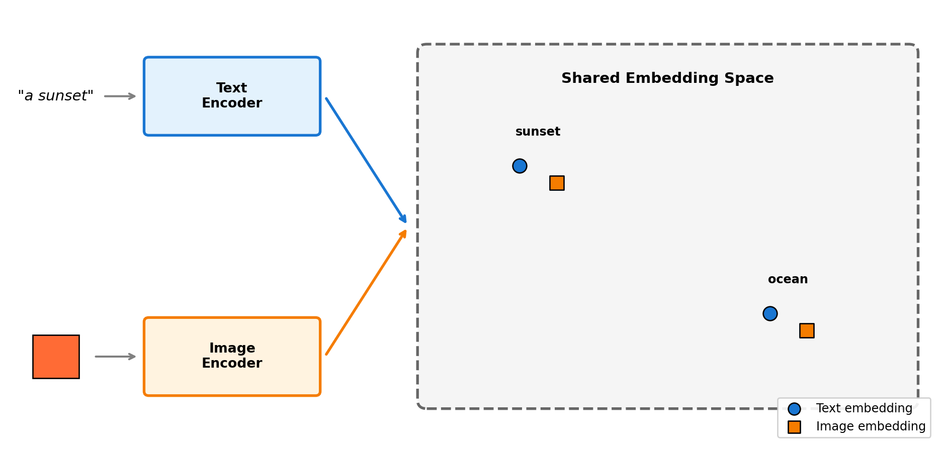
Multi-modal embeddings map different data types—text, images, audio—into a shared vector space where they can be directly compared. This enables powerful cross-modal capabilities: searching images with text queries, finding text descriptions for images, or categorizing images without any training examples.
NoteZero-Shot Categorization via Embeddings
Zero-shot categorization means assigning categories the model was never explicitly trained on—and it works through embedding similarity, not a traditional classifier. Instead of training a “sunset vs ocean vs forest” classifier, you describe categories in text (“a photo of a sunset”), embed both the text and image, and find the closest match. The model generalizes from its pre-training on millions of image-text pairs to recognize new concepts. This is sometimes called “zero-shot classification,” but the mechanism is pure embedding similarity.
The key insight is training two encoders (e.g., one for text, one for images) so that matching pairs produce similar vectors. CLIP, trained on 400 million image-text pairs from the internet, learns that “a photo of a cat” and an actual cat photo should have nearby embeddings:
"""
Multi-Modal Embeddings with CLIP: Zero-Shot Image Categorization

CLIP embeds text and images into the same 512-dimensional space.
We can categorize images by comparing them to text descriptions—
no training on the target categories required.
"""

import torch
import numpy as np
from PIL import Image
from transformers import CLIPProcessor, CLIPModel
from sklearn.metrics.pairwise import cosine_similarity
import warnings
import logging

# Suppress download progress and warnings
logging.getLogger("transformers").setLevel(logging.ERROR)
warnings.filterwarnings("ignore")

# Load CLIP model (downloads ~600MB on first run)
model = CLIPModel.from_pretrained("openai/clip-vit-base-patch32")
processor = CLIPProcessor.from_pretrained("openai/clip-vit-base-patch32", use_fast=True)

# Create test images with distinct characteristics
np.random.seed(42)
images = {
    'sunset': Image.fromarray(
        np.random.randint([200, 100, 50], [255, 150, 100], (224, 224, 3), dtype=np.uint8)
    ),
    'ocean': Image.fromarray(
        np.random.randint([30, 80, 150], [80, 150, 220], (224, 224, 3), dtype=np.uint8)
    ),
    'forest': Image.fromarray(
        np.random.randint([20, 80, 20], [80, 150, 80], (224, 224, 3), dtype=np.uint8)
    ),
}

# Text descriptions to match against
text_labels = [
    "a photo of a sunset with warm orange colors",
    "a photo of the ocean with blue water",
    "a photo of a green forest",
]

# Preprocess: resize images and tokenize text into tensors the model expects
image_inputs = processor(images=list(images.values()), return_tensors="pt", padding=True)
text_inputs = processor(text=text_labels, return_tensors="pt", padding=True)

# torch.no_grad() disables gradient computation since we're only generating
# embeddings, not training. This saves memory and speeds up computation.
with torch.no_grad():
    # Each encoder maps its input to a 512-dim vector in the shared space
    image_embeds = model.get_image_features(**image_inputs).numpy()
    text_embeds = model.get_text_features(**text_inputs).numpy()

# Compare each image embedding to each text embedding using cosine similarity.
# High similarity = the image and text describe the same concept.
similarities = cosine_similarity(image_embeds, text_embeds)

# Zero-shot = categorize without training on these specific categories
# We compare image embeddings to text embeddings and pick the closest match
print("Zero-shot categorization: matching images to text descriptions\n")
print(f"Embedding dimension: {image_embeds.shape[1]}\n")

for i, img_name in enumerate(images.keys()):
    best_match = text_labels[similarities[i].argmax()]
    print(f"{img_name:8} → {best_match}")
    print(f"          scores: {[f'{s:.2f}' for s in similarities[i]]}\n")
Zero-shot categorization: matching images to text descriptions
Embedding dimension: 512
sunset → a photo of a sunset with warm orange colors
scores: ['0.25', '0.20', '0.21']
ocean → a photo of the ocean with blue water
scores: ['0.18', '0.27', '0.22']
forest → a photo of a green forest
scores: ['0.17', '0.22', '0.28']
Show image and embedding visualization code
import matplotlib.pyplot as plt
import matplotlib.gridspec as gridspec

fig = plt.figure(figsize=(10, 3.5))
gs = gridspec.GridSpec(1, 3, wspace=0.3)

for idx, (name, img) in enumerate(images.items()):
    ax = fig.add_subplot(gs[0, idx])
    ax.imshow(img)
    ax.set_title(f'{name.title()}', fontsize=11, fontweight='bold')

    # Show similarity scores below
    scores_text = '\n'.join([f'{text_labels[j].split("of ")[-1][:20]}: {similarities[idx][j]:.2f}'
                             for j in range(len(text_labels))])
    ax.set_xlabel(scores_text, fontsize=9)
    ax.set_xticks([])
    ax.set_yticks([])

plt.suptitle('CLIP matches images to text descriptions via shared embeddings', fontsize=11, fontweight='bold')
plt.subplots_adjust(top=0.85)
plt.show()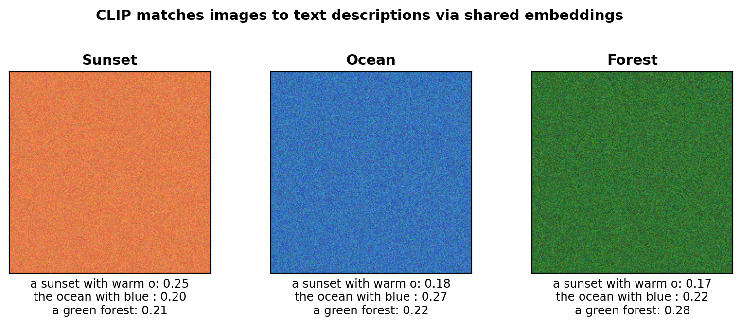
The key insight is that CLIP learns a shared space where semantically matching content—regardless of modality—has similar embeddings. The “sunset” image has warm orange pixels, and CLIP places it near the text “sunset with warm orange colors” because it learned this association from millions of image-text pairs. This enables zero-shot categorization: to categorize an image, compare it against text embeddings and pick the highest similarity—no training on your specific categories required.
When to use multi-modal embeddings: Cross-modal search (text→image, image→text), zero-shot image categorization, image captioning, visual question answering, and product search with text and images.
This book covers multi-modal search in Chapter 12. If you’d like to see other multi-modal applications covered in future editions, reach out to the author.
Popular architectures:
| Architecture | Type | Strengths | Use Cases |
|---|---|---|---|
| CLIP | Text-image | Fast, versatile | Search, classification |
| BLIP-2 | Text-image | Captioning + retrieval | Image understanding |
| ImageBind | 6 modalities | Audio, depth, thermal | Multi-sensor fusion |
| LLaVA | Vision-language | Conversational | Visual Q&A |
6.2 Advanced: Multi-Modal Fusion Strategies
NoteOptional Section
This section covers advanced techniques for combining modalities. Skip if you just need basic multi-modal capabilities.
When working with multiple modalities, you can combine embeddings in several ways:
6.2.1 Early Fusion
Combine embeddings before indexing:
def early_fusion(text_emb, image_emb, weights=(0.5, 0.5)):
    """Combine modalities into a single embedding."""
    fused = weights[0] * text_emb + weights[1] * image_emb
    return fused / np.linalg.norm(fused)  # Normalize
Best for: Static entities where all modalities are always available (products with descriptions and images).
6.2.2 Late Fusion
Combine similarity scores after separate retrieval:
def late_fusion(query_embs, candidate_embs, weights):
    """Combine similarity scores from multiple modalities."""
    total_score = 0
    for modality, weight in weights.items():
        if modality in query_embs:
            score = cosine_similarity(query_embs[modality], candidate_embs[modality])
            total_score += weight * score
    return total_score
Best for: Queries where available modalities vary (user might search with text only, or text + image).
6.2.3 Attention Fusion
Learn which modalities to emphasize for each query:
def attention_fusion(modality_embeddings):
    """Dynamically weight modalities using attention."""
    stacked = torch.stack(modality_embeddings)
    attention_weights = torch.softmax(
        torch.matmul(stacked, stacked.transpose(0, 1)), dim=-1
    )
    attended = torch.matmul(attention_weights, stacked)
    return attended.mean(dim=0)
Best for: Complex queries where modality importance varies by context.
6.3 Key Takeaways
- Multi-modal embeddings create a shared space where different data types (text, images, audio) can be directly compared
- Zero-shot classification works by comparing embeddings to text descriptions—no training on specific categories required
- CLIP is the most popular approach, trained on 400M image-text pairs to align visual and textual concepts
- Fusion strategies determine how to combine modalities: early (before indexing), late (after retrieval), or attention-based (learned weighting)
6.4 Looking Ahead
Now that you understand multi-modal embeddings, Chapter 7 explores graph embeddings—representations that capture network structure and relationships.
6.5 Further Reading
- Radford, A., et al. (2021). “Learning Transferable Visual Models From Natural Language Supervision.” arXiv:2103.00020
- Li, J., et al. (2023). “BLIP-2: Bootstrapping Language-Image Pre-training with Frozen Image Encoders and Large Language Models.” ICML
- Girdhar, R., et al. (2023). “ImageBind: One Embedding Space To Bind Them All.” CVPR