Stacking the blocks to build a complete Decoder-only Transformer
We have spent the last six blogs building individual components:
L01: Tokenizers (Text to IDs)
L02: Embeddings & Positional Encodings (IDs to Vectors + Order)
L03-04: Multi-Head Attention (Understanding Context)
L05: LayerNorm & Residuals (Stability)
L06: Causal Masking (No Cheating)
Now, we wrap them all into a single class. A GPT is essentially a stack of “Transformer Blocks” followed by a final linear layer that maps our vectors back into the vocabulary space to predict the next word.
By the end of this post, you’ll understand:
The structure of a single Transformer Block.
How to stack blocks to create “depth.”
How the final Linear Head produces probabilities for the next token.
Part 1: The Transformer Block
A single block in a GPT model has two main sections:
Communication: The Multi-Head Attention layer where tokens talk to each other.
Computation: A Feed-Forward Network (an MLP!) where each token processes its new information individually.
Each section is wrapped in a Residual Connection and Layer Normalization.
The Feed-Forward Network (FFN) - The “Thinking Step”
After tokens gather context from each other via attention, each token needs to process that information independently. This is where the FFN comes in.
Structure:
nn.Sequential(
    nn.Linear(d_model, 4 * d_model),  # Expand
    nn.ReLU(),                         # Non-linearity
    nn.Linear(4 * d_model, d_model),  # Compress
)
Why the 4× expansion?
The middle layer has 4 times more neurons than the input (e.g., 512 → 2048 → 512)
This creates a “bottleneck” architecture: expand → process → compress
The expansion gives the network more “space” to compute complex transformations
Think of it as giving each token a larger “working memory” for its computations
Purpose:
Attention is about gathering information (communication between tokens)
FFN is about processing that information (independent computation per token)
The FFN applies the same transformation to each position independently—no interaction between tokens
Intuition: After attention, each token has updated its representation based on context. The FFN is like saying: “Now that you know what’s around you, think deeply about what you’ve learned and update your representation accordingly.”
Part 2: The Complete Architecture - Layer by Layer
If we look at the model from top to bottom, it looks like a factory assembly line. Here’s the complete data flow:
The Full GPT Architecture
Key Components Explained:
Token Embedding: Converts integer IDs into dense vectors
Positional Encoding: Adds position information (either sinusoidal or learned)
N Transformer Blocks: Each block refines the representation (typical N = 12, 24, or 96)
Final LayerNorm: One last normalization before prediction
LM Head: Projects back to vocabulary space to predict next token
Part 3: Visualizing the “Hidden States”
As data moves through the blocks, each token’s vector changes. We call these Hidden States.
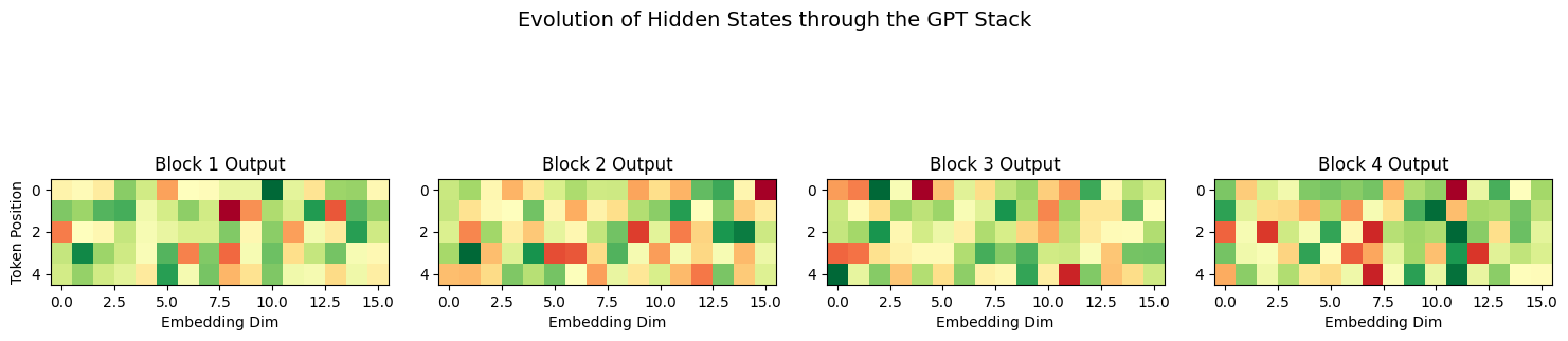
Understanding the Magnitude Decrease
Notice in the visualization above how the values become smaller (less variance) as we move through deeper layers. This isn’t a bug—it’s an expected and important phenomenon!
Why does magnitude decrease?
Layer Normalization: Each LayerNorm operation (used twice per block) forces the mean to 0 and standard deviation to 1. Across many layers, this has a dampening effect on extreme values.
Residual Connections: While they help with gradient flow, they also mean that changes accumulate gradually rather than dramatically. Each layer adds a small delta to the input.
Attention Smoothing: The softmax in attention creates weighted averages. Averaging tends to reduce extreme values and create smoother distributions.
Is this good or bad?
Good! This is actually desirable:
Stability: Bounded values prevent numerical overflow/underflow
Generalization: The model learns robust, stable representations rather than memorizing with extreme activations
Training: Gradients remain in a reasonable range, making optimization more stable
The key insight: The final LayerNorm before the LM head rescales these values appropriately before making predictions. The model learns to work within this normalized regime.
What to watch for: If magnitudes approach zero or if all activations look identical, that could indicate a problem (dead neurons, vanishing gradients). But gradual decrease with maintained structure is healthy.
Part 4: Implementation in PyTorch
Let’s assemble the GPT class. Note how we use nn.ModuleList to stack our blocks.
class TransformerBlock(nn.Module):
    def __init__(self, d_model, n_heads):
        super().__init__()
        self.ln1 = nn.LayerNorm(d_model)
        self.attn = MultiHeadAttention(d_model, n_heads)
        self.ln2 = nn.LayerNorm(d_model)
        self.ff = nn.Sequential(
            nn.Linear(d_model, 4 * d_model),
            nn.ReLU(),
            nn.Linear(4 * d_model, d_model),
        )

    def forward(self, x):
        # Communication (with Residual)
        x = x + self.attn(self.ln1(x))
        # Computation (with Residual)
        x = x + self.ff(self.ln2(x))
        return x

class GPT(nn.Module):
    def __init__(self, vocab_size, d_model, n_layers, n_heads, max_len):
        super().__init__()
        self.token_embedding = nn.Embedding(vocab_size, d_model)
        self.pos_embedding = nn.Parameter(torch.zeros(1, max_len, d_model))

        self.blocks = nn.ModuleList([
            TransformerBlock(d_model, n_heads) for _ in range(n_layers)
        ])

        self.ln_final = nn.LayerNorm(d_model)
        self.lm_head = nn.Linear(d_model, vocab_size)

    def forward(self, idx):
        b, t = idx.size()
        x = self.token_embedding(idx) + self.pos_embedding[:, :t, :]

        for block in self.blocks:
            x = block(x)

        x = self.ln_final(x)
        logits = self.lm_head(x) # Scores for every word in the vocab
        return logits
Summary
The Stack: We build a deep model by repeating the Transformer Block.
Hidden States: Each layer refine’s the token’s meaning based on context.
The Head: The final layer is just a classifier that asks: “Based on everything I’ve seen, which token comes next?”
Next Up: L08 – Architecture Design Choices. Now that you know how to build a GPT, we need to decide on the hyperparameters: How many layers? How many attention heads? What embedding dimension? We’ll explore how to design your architecture for different use cases.