How to talk to a trained brain without it repeating itself
We have a trained GPT model from L08 - Training the LLM. If we give it a prompt, the model will output a list of probabilities for the next word.
This post covers the “magic” of how an LLM actually generates text. Training is about building a probability map; Inference is about walking through that map. We will also explore the “knobs” we turn to make the model more creative or more factual.
But how do we choose the “best” word? If we always pick the most likely word (Greedy Search), the model often gets stuck in a loop, repeating the same phrase over and over. To make the model sound human, we need to introduce a bit of randomness.
By the end of this post, you’ll understand:
The Autoregressive Loop (generating one word at a time).
How Temperature affects the “sharpness” of probabilities.
Advanced techniques like Top-K and Top-P (Nucleus) sampling.
Part 1: The Autoregressive Loop
Generating text is a loop. The model predicts one token, we append that token to the input, and we feed the new, longer sequence back into the model to get the next token.
Prompt: “The cat”
Model predicts: “sat” (Prob: 0.8)
New Input: “The cat sat”
Model predicts: “on” (Prob: 0.7)
Repeat until a special “End of Sentence” token is generated.
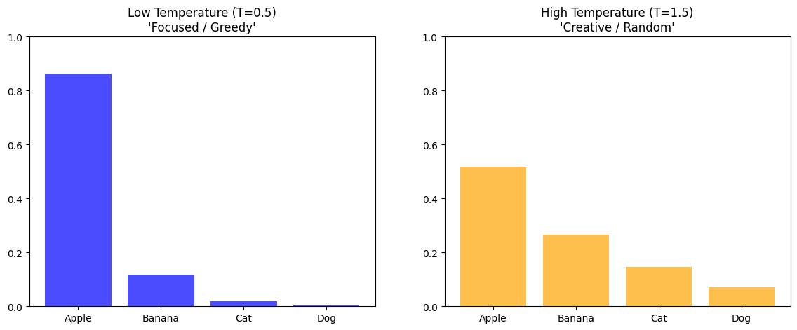
Part 2: Temperature (The “Creativity” Knob)
Before we pick a word, we can “stretch” or “squash” the probability distribution using Temperature (T).
We divide the raw scores (logits) by T before the Softmax:
Low Temperature (T < 1): Makes the high probabilities higher and low ones lower. The model becomes very confident and “boring” (Greedy).
High Temperature (T > 1): Flattens the distribution. Rare words get a higher chance of being picked. The model becomes “creative” but potentially nonsensical.
Part 3: Top-K & Top-P Sampling
Even with temperature, sometimes the model picks a word that is just objectively wrong (like a low chance word). To prevent this, we use filters:
Top-K Sampling
We only look at the top K most likely words and ignore everything else. This keeps the model from “veering off the rails.”
Top-P (Nucleus) Sampling
Instead of a fixed number of words, we pick the smallest set of words whose cumulative probability adds up to P (e.g., 0.9). This is more dynamic; if the model is very sure, it might only look at 2 words. If it’s unsure, it might look at 20.
Concrete Example:
Suppose after applying temperature=1.0 to our logits and running softmax, we get these probabilities:
| Token | Probability | Cumulative Probability |
|---|---|---|
| “the” | 0.40 | 0.40 |
| “a” | 0.30 | 0.70 |
| “this” | 0.20 | 0.90 ← Cutoff at p=0.9 |
| “that” | 0.05 | 0.95 |
| “my” | 0.03 | 0.98 |
| “your” | 0.02 | 1.00 |
With top_p = 0.9:
Sort tokens by probability (already sorted above)
Add probabilities until we reach 0.9: “the” (0.40) + “a” (0.30) + “this” (0.20) = 0.90
Keep only these 3 tokens:
["the", "a", "this"]Renormalize: divide each by the sum (0.90) to get a proper probability distribution
Sample from this smaller set
Result: The model can only choose from “the”, “a”, or “this”—cutting off the unlikely tokens “that”, “my”, and “your.”
Why it’s better than top-k:
Adaptive: When the model is confident (one token has 0.95 probability), nucleus might only keep that 1 token. When uncertain (many tokens around 0.1 each), it keeps more options.
Quality-based: Cuts based on probability mass, not arbitrary count
Visualizing Top-P Filtering:
/tmp/ipykernel_5217/2216869106.py:32: UserWarning: set_ticklabels() should only be used with a fixed number of ticks, i.e. after set_ticks() or using a FixedLocator.
  ax1.set_xticklabels(tokens, rotation=45)
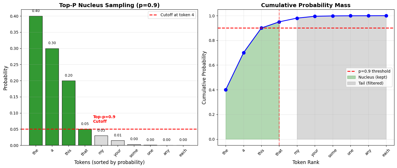
Key insight from the visualization:
Left plot: Only the first 3 tokens (green) are kept—they account for 90% of probability mass
Right plot: Cumulative probability curve crosses the 0.9 threshold after 3 tokens
The remaining 7 tokens (gray) are filtered out despite being possible candidates
This adaptive filtering keeps quality high while allowing flexibility when the model is uncertain.
Part 4: The Inference Code
Here is how we implement the generation loop in PyTorch, including a simple temperature adjustment.
@torch.no_grad()
def generate(model, idx, max_new_tokens, temperature=1.0, top_k=None):
    for _ in range(max_new_tokens):
        # 1. Crop idx to the last 'block_size' tokens
        idx_cond = idx[:, -block_size:]

        # 2. Forward pass to get logits
        logits = model(idx_cond)

        # 3. Focus only on the last time step and scale by temperature
        logits = logits[:, -1, :] / temperature

        # 4. Optional: Top-K filtering
        if top_k is not None:
            v, _ = torch.topk(logits, top_k)
            logits[logits < v[:, [-1]]] = -float('Inf')

        # 5. Softmax to get probabilities
        probs = F.softmax(logits, dim=-1)

        # 6. Sample from the distribution
        idx_next = torch.multinomial(probs, num_samples=1)

        # 7. Append to the sequence
        idx = torch.cat((idx, idx_next), dim=1)

    return idx
Part 5: Advanced Sampling Techniques
max_new_tokens - Controlling Generation Length
The max_new_tokens parameter determines how many tokens the model will generate:
generated = generate(model, prompt, max_new_tokens=50)What it does:
Limits the generation loop to exactly 50 iterations
After 50 tokens, generation stops regardless of content
Prevents infinite loops and controls costs (API calls are often priced per token)
How models know when to stop naturally:
Models learn to generate special end-of-sequence tokens (like
<|endoftext|>)When the model generates this token, we can stop early (before hitting max_new_tokens)
During training, these tokens appear at document boundaries
Typical values:
Chatbots: 512-2048 tokens (one response)
Code completion: 100-500 tokens (one function)
Creative writing: 1000-4096 tokens (longer passages)
Repetition Penalty - Preventing Loops
A common problem: models get stuck repeating the same phrase:
"The cat sat on the mat. The cat sat on the mat. The cat sat on..."Solution: Repetition Penalty
def apply_repetition_penalty(logits, previous_tokens, penalty=1.2):
    for token in set(previous_tokens):
        # Divide logit by penalty (reduces probability)
        logits[token] /= penalty
    return logits
How it works:
Track all previously generated tokens
Before sampling, reduce the logits of tokens that already appeared
penalty > 1.0makes repetition less likelypenalty = 1.0means no penalty (default behavior)
Typical values:
penalty = 1.0: No penalty (may repeat)penalty = 1.2: Mild discouragement of repetition (balanced)penalty = 1.5: Strong avoidance (may sound unnatural)
Beam Search - Deterministic Exploration
All the sampling methods above are stochastic (random). Beam Search is a deterministic alternative:
How it works:
Instead of sampling 1 token, keep the top
beam_widthcandidatesFor each candidate, generate the next token
Evaluate all
beam_width²possibilitiesKeep only the top
beam_widthsequences by total probabilityRepeat until done
Example with beam_width=2:
Start: "The"
Step 1: Keep ["The cat" (prob=0.8), "The dog" (prob=0.7)]
Step 2: Expand both → ["The cat sat" (0.64), "The cat ran" (0.56),
                       "The dog sat" (0.49), "The dog ran" (0.42)]
        Keep top 2 → ["The cat sat", "The cat ran"]
... continue ...
Beam Search vs. Sampling:
| Aspect | Beam Search | Sampling (Top-P/Top-K) |
|---|---|---|
| Determinism | Always same output | Different every time |
| Quality | Finds high-probability sequences | More diverse, creative |
| Use cases | Translation, summarization | Creative writing, chat |
| Speed | Slower (beam_width parallel paths) | Faster (single path) |
When to use:
Beam search: When you want the “safest” or most likely output (translation, factual Q&A)
Sampling: When you want variety and creativity (storytelling, brainstorming)
Summary
Inference is a loop where the model’s output becomes its next input.
Temperature controls how much the model deviates from its most likely guess (sharpness of distribution).
Sampling Strategies (Top-K/Top-P) prune the “long tail” of unlikely words to maintain coherence.
max_new_tokens controls generation length and prevents runaway generation.
Repetition Penalty prevents the model from getting stuck in loops by penalizing already-used tokens.
Beam Search offers a deterministic alternative to sampling, finding high-probability sequences for tasks requiring consistency.
Next Up: L10 – Fine-tuning (RLHF & Chat). We have a model that can complete sentences. But how do we turn it into a helpful assistant that answers questions? We’ll look at the final step: taking a “Base” model and turning it into a “Chat” model.