Vectors#
Introduction#
Welcome to the fundamentals of linear algebra! This section will introduce you to the basic concepts and operations that are essential for understanding linear algebra. Whether you’re new to the subject or looking to refresh your knowledge, this guide will help you grasp the core ideas through both theoretical explanations and practical examples.
Definition: Vector
We begin with the basics of vectors. A vector in mathematics is an object that has both magnitude and direction. In the context of linear algebra, vectors are essential building blocks used in various operations and applications.
2D Vector#
First start with 2D to keep concepts simple for understanding basic functionality.
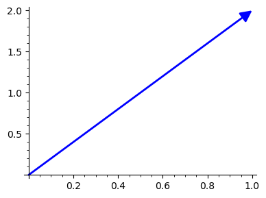
v = vector([1,2])
type(v)
<class 'sage.modules.vector_integer_dense.Vector_integer_dense'>
Sagemath vector() docs: sage.modules.vector_integer_dense.Vector_integer_dense
Graphics#
Plot our vector.
v.plot(figsize=4)
Sagemath Graphics docs: sage.plot.graphics.Graphics
Linear Combinations#
The linear combination of the vectors \(𝐯_1,𝐯_2,…,𝐯_𝑛\) with scalars \(𝑐_1,𝑐_2,…,𝑐_𝑛\) is the vector
\(𝑐_1𝐯_1+𝑐_2𝐯_2+…+𝑐_𝑛𝐯_𝑛.\)
The scalars \(𝑐_1,𝑐_2,…,𝑐_𝑛\) are called the weights of the linear combination.
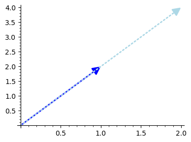
Scalar multiplication#
v1 = vector([1,2])
c1 = 2

v1xc1 = c1*v1

plots = v1.plot(color='blue') + v1xc1.plot(color='lightblue', linestyle=':')
show(plots, figsize=4)
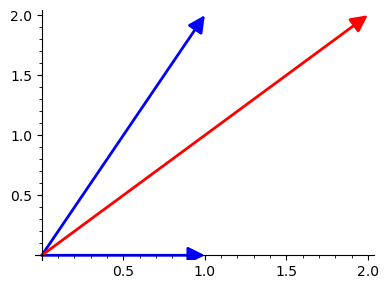
Vector addition#
v1 = vector([1,2])
v2 = vector([1,0])

v1_v2 = v1 + v2

plots = v1.plot(color='blue') + v2.plot(color='blue') + v1_v2.plot(color='red')
show(plots, figsize=4)
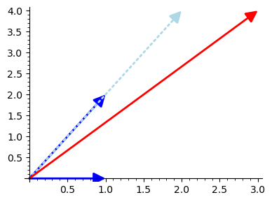
Scalar multiplication and Vector Addition “Combined”#
Linear Combination = both Scalar multiplication and Vector Addition
v1 = vector([1,2])
c1 = 2

v2 = vector([1,0])
c2 = 1

lin_combination = c1*v1 + c2*v2

plots = \
    v1.plot(color='blue') + \
    (c1*v1).plot(color='lightblue', linestyle=':') + \
    v2.plot(color='blue') + \
    lin_combination.plot(color='red')

show(plots, figsize=4)
n-Dim Vectors#
Let’s extend to 3D to
r = vector([1,2,0])
s = vector([-1,4,0])
vplot = r.plot(color='red',ticks=0.25) + s.plot(color='green')

# the following code only works when the notebook is run in the sagemath environment
show(vplot, gridlines='major', )
(You can interactively rotate, zoom, and pan the above 3D plots using the mouse)