Transformations#
Let’s dive into linear transformations using SageMath code and visualizations.
Core Concepts#
Definitions: Linear transformations
Linear transformations (or maps) are functions that take vectors from one vector space and transform them into vectors in another (or potentially the same) vector space (e.g. 3D \(\rightarrow\) 2D, 3D \(\rightarrow\) 3D, etc). They obey two key rules:
Additivity: T(u + v) = T(u) + T(v) (The transformation of a sum is the sum of the transformations)
Homogeneity: T(cu) = cT(u) (Scaling a vector before transforming is the same as scaling after)
Linear transformations are fundamental to many fields:
Geometry: They describe rotations, reflections, stretches, shears, etc.
Physics: They represent changes in physical systems over time or space.
Data Science: They underlie dimensionality reduction techniques (PCA, etc.).
Linear transformations are often represented by matrices. Applying the transformation means multiplying the matrix by a vector.
SageMath Code Examples
Example 1. Basic transformation#
Step 1: Define the transformation matrix \( A \):
\( A = \begin{pmatrix} 2 & 1 \\ 1 & 3 \\ \end{pmatrix} \)
Step 2: Define the vector to be transformed \(\mathbf{v}\):
\( \mathbf{v} = \begin{pmatrix} 1 \\ 0 \\ \end{pmatrix} \)
Step 3: Apply the transformation \( \mathbf{w} \):
\( \mathbf{w} = A \cdot \mathbf{v} \)
Step 4: Calculate \( \mathbf{w} \):
\( \mathbf{w} = \begin{pmatrix} 2 & 1 \\ 1 & 3 \\ \end{pmatrix} \cdot \begin{pmatrix} 1 \\ 0 \\ \end{pmatrix} \)
Step 5: Simplify the result:
\( \mathbf{w} = \begin{pmatrix} 2 \cdot 1 + 1 \cdot 0 \\ 1 \cdot 1 + 3 \cdot 0 \\ \end{pmatrix} = \begin{pmatrix} 2 \\ 1 \\ \end{pmatrix} \)
Step 6: Display the vector before and after transformation:
\( \text{Vector before transformation: } \begin{pmatrix} 1 \\ 0 \\ \end{pmatrix} \)
\( \text{Vector after transformation: } \begin{pmatrix} 2 \\ 1 \\ \end{pmatrix} \)
These steps outline the process of applying the linear transformation matrix \( A \) to the vector \( \mathbf{v} \) and obtaining the transformed vector \( \mathbf{w} \).
Here is the SageMath code:
# Define a transformation matrix
A = matrix([[2, 1],
            [1, 3]])

# Define a vector before transformation
v = vector([1, 0])

# Apply the transformation
w = A * v

# Display the vector before and after transformation
print("Vector before transformation:", v)
print("Vector after transformation:", w)
Vector before transformation: (1, 0)
Vector after transformation: (2, 1)
Example 2. Rotation Transformation#
Let’s create a linear transformation that rotates vectors in the 2D plane by 45 degrees counter-clockwise.
# Define standard basis vectors
e1 = vector(RDF, [1, 0])
e2 = vector(RDF, [0, 1])

# Plot the standard basis vectors
p = arrow((0, 0), e1, color='blue', arrowsize=2.0) + \
    arrow((0, 0), e2, color='blue', arrowsize=2.0)

# Define the transformation matrix
A = matrix(RDF, [[2, 1], [1, 2]])

# Apply the transformation to the basis vectors
Te1 = A * e1
Te2 = A * e2
p += arrow((0, 0), Te1, color='red', arrowsize=2) + \
     arrow((0, 0), Te2, color='red', arrowsize=2)

# Create a square and apply the transformation
square_points = [vector(RDF, [1, 1]),
                 vector(RDF, [1, -1]),
                 vector(RDF, [-1, -1]),
                 vector(RDF, [-1, 1]),
                 vector(RDF, [1, 1])]

Tsquare = [A * point for point in square_points]

# Plot the square and its transformation
p += line(square_points, color='green') + line(Tsquare, color='green')

# Add labels (with spacing)
p += text("$e_1$", (e1[0] + 0.2, e1[1] + 0.1), fontsize=12, color='blue')
p += text("$e_2$", (e2[0] + 0.2, e2[1] + 0.1), fontsize=12, color='blue')
p += text("$T(e_1)$", (Te1[0] - 0.3, Te1[1] + 0.2), fontsize=12, color='red')
p += text("$T(e_2)$", (Te2[0] - 0.3, Te2[1] + 0.2), fontsize=12, color='red')

# Show the plot with gridlines and adjust plot settings

p.show(aspect_ratio=1, xmin=-3, xmax=3, ymin=-3, ymax=3, gridlines=True)
In this example we use RDF to give you some exposure to other field types.
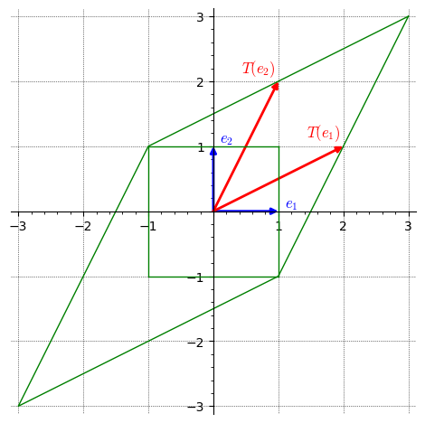
This code snippet begins by defining the standard basis vectors, \( \mathbf{e_1} \) and \( \mathbf{e_2} \), in a two-dimensional vector space over the real numbers. These vectors serve as the fundamental building blocks for representing other vectors and transformations.
Next, a transformation matrix \( A \) is created to represent a 45-degree counter-clockwise rotation. This matrix captures the effect of the rotation on vectors in the vector space.
The transformation \( A \) is then applied to the standard basis vectors \( \mathbf{e_1} \) and \( \mathbf{e_2} \) to obtain the transformed vectors \( T(\mathbf{e_1}) \) and \( T(\mathbf{e_2}) \), respectively. These transformed vectors illustrate how the rotation affects the original basis vectors.
A unit square is constructed using a set of points, and the transformation \( A \) is applied to each point of the square. This results in a new set of points representing the transformed square after the rotation.
The plot displays the original unit vectors \( \mathbf{e_1} \) and \( \mathbf{e_2} \) in blue, their transformed counterparts \( T(\mathbf{e_1}) \) and \( T(\mathbf{e_2}) \) in red, and the unit square along with its transformation in green. Additionally, labels are added to visually identify the vectors.
The plot settings are adjusted to ensure proper scaling and visibility, with gridlines included to aid in visualization.
Overall, this code provides a visual representation of a linear transformation in two dimensions, showcasing the rotation of vectors and shapes using matrix operations.
Visualization Insights
Rotation Effect: You’ll see how the original square (in green) is rotated counter-clockwise by 45 degrees, resulting in a diamond shape (in green).
Connection to Matrix Operations: The visualization directly connects the geometric transformation to the matrix multiplication operation.
Identity Matrix#
Definitions: Identity Matrix
In linear algebra, the identity matrix is a square matrix denoted as \( I \) or \( I_n \), where \( n \) represents its dimension. It has 1s along the main diagonal and 0s elsewhere. For example:
\( I_2 = \begin{pmatrix} 1 & 0 \\ 0 & 1 \end{pmatrix} \)
\( I_3 = \begin{pmatrix} 1 & 0 & 0 \\ 0 & 1 & 0 \\ 0 & 0 & 1 \end{pmatrix} \)
This matrix, when multiplied with any other matrix, yields the same matrix—a property crucial in various matrix operations.
# Define the 2x2 identity matrix
I_2 = matrix.identity(2)

# Define a vector
v = vector([2, 3])

# Apply the identity transformation
v_identity = I_2 * v

# Display the original and transformed vectors
print("Original vector:", v)
print("Vector after identity transformation:", v_identity)
Original vector: (2, 3)
Vector after identity transformation: (2, 3)
Inverse Matrix#
Definitions: Inverse Matrix
The inverse of a square matrix \( A \), denoted as \( A^{-1} \), is another matrix such that when multiplied by \( A \), yields the identity matrix \( I \). Mathematically:
\( A \cdot A^{-1} = A^{-1} \cdot A = I \)
In linear transformations, the inverse matrix reverses the effects of a transformation. For instance, if \( A \) transforms a vector \( \mathbf{v} \) into \( \mathbf{v'} \), then \( A^{-1} \) can revert \( \mathbf{v'} \) back to \( \mathbf{v} \) by multiplying it.
See the section Extra Content - manually finding a matrix inverse at the end of this notebook if you want to manually find a matrix inverse.
Here’s a 2D example of a transformation matrix and its inverse represented in LaTeX:
Original matrix \( A \) representing a transformation:
\( A = \begin{pmatrix} 2 & 1 \\ 1 & 2 \end{pmatrix} \)
Inverse matrix \( A^{-1} \) to reverse the transformation:
\( A^{-1} = \begin{pmatrix} \frac{2}{3} & -\frac{1}{3} \\ -\frac{1}{3} & \frac{2}{3} \end{pmatrix} \)
In this example, \( A \) represents a linear transformation, and \( A^{-1} \) reverses this transformation when applied to the transformed vectors.
# Define the 2x2 transformation matrix
A = matrix([[2, 1],
            [1, 2]])

# Compute the inverse of A
A_inv = A.inverse()

# Define a vector before transformation
v_before = vector([3, 4])

print("Original vector before transformation:", v_before)
Original vector before transformation: (3, 4)
# Apply the transformation
v_after = A * v_before

print("Vector after transformation:", v_after)
Vector after transformation: (10, 11)
# Apply the inverse transformation
v_back = A_inv * v_after

print("Vector after inverse transformation:", v_back)
Vector after inverse transformation: (3, 4)
Exercises#
Here are some ideas to explore transformations further:
Different Transformations: Experiment with other transformation matrices to visualize reflections, stretches, shears, etc.
More Complex Shapes: Apply the transformation to triangles, polygons, or even curves to see how they are affected.
Higher Dimensions: SageMath can handle 3D and higher-dimensional transformations. Try visualizing how a cube is transformed in 3D space.
Extra Content - manually finding a matrix inverse#
To find the inverse of a 2x2 matrix like A = [[2, 1], [1, 2]], you can use the following formula:
\( A^{-1} = \frac{1}{{ad - bc}} \times \begin{bmatrix} d & -b \\ -c & a \end{bmatrix} \)
Where \( a \), \( b \), \( c \), and \( d \) are the elements of the matrix A, and \( ad - bc \) is the determinant of A.
For the matrix A = [[2, 1], [1, 2]], we have:
\( a = 2, \quad b = 1, \quad c = 1, \quad d = 2 \)
The determinant of A is:
\( ad - bc = (2 \times 2) - (1 \times 1) = 3 \)
Now, plug these values into the formula to find the inverse:
\( A^{-1} = \frac{1}{3} \times \begin{bmatrix} 2 & -1 \\ -1 & 2 \end{bmatrix} \)
\( A^{-1} = \frac{1}{3} \times \begin{bmatrix} 2 & -1 \\ -1 & 2 \end{bmatrix} \)
\( A^{-1} = \begin{bmatrix} \frac{2}{3} & -\frac{1}{3} \\ -\frac{1}{3} & \frac{2}{3} \end{bmatrix} \)
So, the inverse of the matrix A is:
\( A^{-1} = \begin{bmatrix} \frac{2}{3} & -\frac{1}{3} \\ -\frac{1}{3} & \frac{2}{3} \end{bmatrix} \)