Eingenvalues

Let’s dive into eigenvalues, eigenvectors, and their significance in linear algebra, along with SageMath examples and visualizations.

Introduction

Definitions:

Think of a linear transformation (like stretching, rotating, or reflecting) applied to a vector space. An eigenvector is a special vector that, when the transformation is applied, only changes in magnitude (gets scaled), not direction. The scaling factor associated with that eigenvector is called its eigenvalue.

In simpler terms, eigenvectors are the “invariant directions” under a linear transformation. They point along the axes where the transformation’s effect is most straightforward – just stretching or shrinking.

Geometric Interpretation

Imagine a transformation that stretches a circle into an ellipse. The major and minor axes of the ellipse are the eigenvectors, and how much each axis stretches/shrinks represents the corresponding eigenvalue.

Computation

The process of finding eigenvalues and eigenvectors involves solving the following equation:

A * v = λ * v

where:

• A is a square matrix representing the linear transformation

• v is the eigenvector

• λ (lambda) is the eigenvalue

This equation basically says: “When matrix A acts on vector v, it’s the same as simply scaling vector v by a factor of λ.”

SageMath Examples

Let’s use SageMath to find the eigenvalues and eigenvectors of a matrix:

A = matrix([[3, 1], [2, 2]])
print("Matrix A:\n", A)

eigenvalues, eigenvectors = A.eigenmatrix_right()
print("\nEigenvalues (on the diagonal):\n", eigenvalues)
print("\nEigenvectors (as columns):\n", eigenvectors)

Matrix A:
 [3 1]
[2 2]

Eigenvalues (on the diagonal):
 [4 0]
[0 1]

Eigenvectors (as columns):
 [ 1  1]
[ 1 -2]

Eigenvalues on the Diagonal: The A.eigenmatrix_right() function in SageMath returns a matrix where the eigenvalues are located on the main diagonal. In this case, the diagonal elements are 4 and 1, representing the eigenvalues. Eigenvectors as Columns: The eigenvectors are returned as the columns of the matrix. So, the first eigenvector corresponding to the eigenvalue 4 is [1, 1], and the second eigenvector corresponding to the eigenvalue 1 is [1, -2].

Visualization with SageMath

We can visualize how the transformation defined by matrix A acts on the standard basis vectors and the eigenvectors:

import matplotlib.pyplot as plt

# Original basis vectors
i = vector([1, 0])
j = vector([0, 1])

# Transformed basis vectors
i_transformed = A * i
j_transformed = A * j

# Plot
plt.figure()
plt.quiver([0, 0], [0, 0], [i[0], i_transformed[0]], [i[1], i_transformed[1]], 
           angles='xy', scale_units='xy', scale=1, color='blue', label='i, A*i')

plt.quiver([0, 0], [0, 0], [j[0], j_transformed[0]], [j[1], j_transformed[1]], 
           angles='xy', scale_units='xy', scale=1, color='red', label='j, A*j')


colors = ['green', 'purple']
for i, v in enumerate(eigenvectors.columns()):
    v_transformed = A * v
    plt.quiver([0, 0], [0, 0], [v[0], v_transformed[0]], [v[1], v_transformed[1]], 
               angles='xy', scale_units='xy', scale=1, color=colors[i], 
               label=f'col[{i}] Eigenvector, A*Eigenvector')

plt.xlim(-1, 5)
plt.ylim(-3, 5)
plt.grid()
plt.legend(loc='upper left')
plt.show()

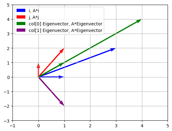
The blue and red quivers in the plot represent the original basis vectors (i and j) and their transformed versions after being multiplied by matrix A.

Let’s break it down:

• Blue Quiver: This represents the standard basis vector i = (1, 0). The blue arrow starts at the origin (0, 0) and ends at the point (1, 0). The transformed version A * i is shown as a blue arrow starting at the origin and ending at the point where i is mapped to by the transformation.

• Red Quiver: This represents the standard basis vector j = (0, 1). The red arrow starts at the origin (0, 0) and ends at the point (0, 1). Similarly, A * j is shown as a red arrow starting at the origin and ending at the point where j is mapped to by the transformation.

Why Show These?

Visualizing the original basis vectors and their transformed versions helps us understand how the linear transformation (represented by matrix A) distorts the space. It gives us a clear picture of how the transformation stretches, rotates, or reflects the standard coordinate axes.

Additional Notes:

• The transformation defined by matrix A in your example seems to stretch the i vector and slightly rotate both i and j.

• The green (and purple, if you used the modified code) quivers represent the eigenvectors and their transformed versions, showcasing how they remain aligned with their original directions under the transformation.

Diagonalization and Applications

If a matrix has enough linearly independent eigenvectors, it can be diagonalized. This means we can express it in a simpler form:

A = P * D * P^(-1)

where:

• P is a matrix whose columns are the eigenvectors

• D is a diagonal matrix with the eigenvalues on the diagonal

Diagonalization is immensely useful in:

• Solving systems of differential equations

• Calculating matrix powers efficiently

• Simplifying calculations in quantum mechanics and other fields