Solution Sets#
Introduction#
In linear algebra, a solution set is the collection of all possible values for variables that satisfy a system of linear equations. A solution set can represent a unique solution, infinitely many solutions, or can be empty, meaning no solutions exist. Solution sets help understand the relationships between equations and characterize the properties of linear systems. It’s called a “set” because it contains all valid solutions for a linear system.
Let’s begin with our augmented RREF matrix from the previous section:
Coefficients: the columns to the left of the vertical bar
Constants: the column to the right of the vertical bar
Pivots: a pivot element is a nonzero element that is the first nonzero entry in its row when using the Gaussian elimination method to convert the matrix into row echelon form or reduced row echelon form
In the above example, we have a pivot in each coefficient column.
SageMath has a method pivots() to return the pivot locations for a matrix:
A = Matrix([[1, 0, 0, 8/9],
            [0, 1, 0, 7/3],
            [0, 0, 1, 14/9]])

A.pivots()
(0, 1, 2)
Determining how many solutions exist#
The following RREF’s show the three types of solutions that are possible:
Unique Solution: a unique solution has a pivot in all coefficient columns
Infinite Solutions: infinite solutions have a row with no pivots
No Solution: there are no solutions if there is a pivot in the constant column
Consistent System: a system of linear equations is considered consistent if it has at least one solution. This means there exists a set of values for the variables that satisfies all equations simultaneously
Let’s elaborate on each of these
Unique Solution#
A = Matrix([[3, -2],[1, 4]])
b = vector([-2,2])

A_aug = A.augment(b, subdivide=True)
show(A_aug)
A_rref = A_aug.rref()
show(A_rref)
A_rref.pivots()
(0, 1)
We have a pivot in each coefficient column so this is a unique solution.
Let’s verify there is only one solution, using solve_right().
A.solve_right(b) # note we are using the A matrix, not the augmented matrix A_aug
(-2/7, 4/7)
The solution to this linear system is:
\(x = -2/7\)
\(y = 4/7\)
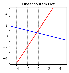
If we plot the linear system, we can see that the lines meet at exactly one point \(x = -2/7, y = 4/7\) and is therefore a unique solution.
var('x y')

equation1 = 3*x - 2*y == -2
equation2 = x + 4*y == 2

# Create the plots using implicit_plot
plot1 = implicit_plot(equation1, (x, -5, 5), (y, -5, 5), color='red', gridlines='faint')
plot2 = implicit_plot(equation2, (x, -5, 5), (y, -5, 5), color='blue', gridlines='faint')

# Combine plots and show with intersection point
(plot1 + plot2).show(title='Linear System Plot', figsize=4)
Infinite Solutions#
Let’s start with this linear system.
In this system, if you divide the second equation by 2, you get the first equation. However, the second equation is not a multiple of the first. These equations represent parallel lines with the same slope but different y-intercepts. Since they never intersect, they have infinitely many solutions, meaning any point on one of the lines satisfies both equations.
A = Matrix([[3, 2],[6, 4]])
b = vector([7, 14])

A_aug = A.augment(b, subdivide=True)
show(A_aug)
A_rref = A_aug.rref()
show(A_rref)
A_rref.pivots()
(0,)
We can see that there is only one pivot - for the variable x.
Because there is a row with no pivots this system has infinite solutions.
In this case y is a free variable as it doesn’t have a pivot.
By swapping terms so that \(x\) is dependent on \(y\), we can see that: \(x == -2/3*y + 7/3\)
Definition: Free variable
In linear algebra, a free variable is a variable that can take on any value independently of other variables in a system of linear equations.
When you have an equation like \(x = -\frac{2}{3}y + \frac{7}{3}\), it represents a linear relationship between the variables \(x\) and \(y\). In this equation, \(x\) is expressed in terms of \(y\).
For any real number you choose for \(y\), you can calculate the corresponding value of \(x\) using the given relationship. Therefore, every real number you choose for \(y\) will yield a corresponding solution for \(x\), making the solution set infinite and continuous along a line with slope \(-\frac{2}{3}\) and y-intercept \(\frac{7}{3}\).
Here are two example solutions in this infinite solution set:
Example 1.
Let’s choose \( y = 0 \). Using the equation \( x = -\frac{2}{3}y + \frac{7}{3} \), we can calculate \( x \):
\(x = -\frac{2}{3}(0) + \frac{7}{3} = \frac{7}{3}\) So, when \( y = 0 \), \( x = \frac{7}{3} \). Therefore, one solution is \( (x, y) = \left(\frac{7}{3}, 0\right) \).
Example 2.
Now, let’s choose \( y = 3 \). Using the same equation:
\(x = -\frac{2}{3}(3) + \frac{7}{3} = -2 + \frac{7}{3} = \frac{1}{3}\) So, when \( y = 3 \), \( x = \frac{1}{3} \). Another solution is \( (x, y) = \left(\frac{1}{3}, 3\right) \).
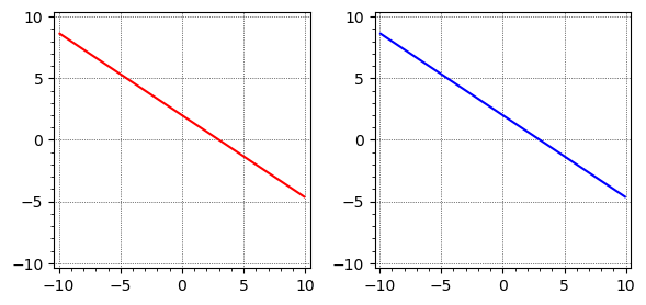
If we plot the linear system, we can see the lines overlap exactly, hence infinite solutions.
# Define the symbolic variables
x, y = var('x y')

# Define the equations
equation1 = 2*x + 3*y == 6
equation2 = 4*x + 6*y == 12

# Create the plots using implicit_plot
plot1 = implicit_plot(equation1, (x, -10, 10), (y, -10, 10), color='red', gridlines='faint')
plot2 = implicit_plot(equation2, (x, -10, 10), (y, -10, 10), color='blue', gridlines='faint')

# Show plots side by side with equation text
(graphics_array([[plot1, plot2]])).show(figsize=6)
No Solution#
A = Matrix([[3, 2],[6, 4]])
b = vector([7,12])

A_aug = A.augment(b, subdivide=True)
show(A_aug)
A_rref = A_aug.rref()
show(A_rref)
There is a pivot is in the constant column so there is no solution.
We can also use the pivots() method to show this.
A_rref.pivots()
(0, 2)
# if there is no solution solve_right raises 'ValueError: matrix equation has no solutions'
try:
    A.solve_right(b) # note we are using the A matrix, not the augmented matrix A_aug
except ValueError:
    print("matrix equation has no solutions")
matrix equation has no solutions
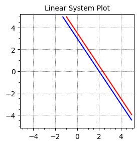
If we plot the linear system, we can see the lines are parallel and will never overlap.
var('x y')

equation1 = 3*x + 2*y == 7
equation2 = 6*x + 4*y == 12

# Create the plots using implicit_plot
plot1 = implicit_plot(equation1, (x, -5, 5), (y, -5, 5), color='red', gridlines='faint')
plot2 = implicit_plot(equation2, (x, -5, 5), (y, -5, 5), color='blue', gridlines='faint')

# Combine plots and show with intersection point
(plot1 + plot2).show(title='Linear System Plot', figsize=4)
Solution automation#
This section shows a utility function for describing solution sets.
def solution_details(augmented_matrix, vars=None):
    try:
        num_coeff_cols = augmented_matrix.subdivisions()[1][0]
        if not num_coeff_cols > 0:
            raise ValueError("Subdivided augmented matrix required.")
    except (AttributeError, IndexError):
        raise ValueError("Subdivided augmented matrix required.")

    pivots = augmented_matrix.pivots()
    const_col = num_coeff_cols + 1

    print("Matrix and RREF:")
    import sys

    u = [augmented_matrix, augmented_matrix.rref()]
    show(augmented_matrix, augmented_matrix.rref())

    print()

    # is RHS all zeros
    is_zero = all(component == 0 for component in augmented_matrix[:, -1])
    if is_zero:
        print('Matrix is homogeneous, must be consistent (always at least one soln - the 0 vector).')
    else:
        print('Matrix is not homogeneous - can be inconsistent.')

    if (const_col - 1) in pivots:
        print('No Solution (Inconsistent - const col has pivot)')
    else:
        if len(pivots) == num_coeff_cols:
            print("Unique Solution (Consistent, pivot position in each col)")
        elif len(pivots) < num_coeff_cols:
            print('Infinitely Many Solutions (Consistent, >= 1 coeff col with no pivots)')

    solution, X, X_pivots, X_free, param_sol_dict = my_solve(augmented_matrix, vars)

    print("Variables: ", X)
    print("Pivots (leading) variables: ", X_pivots)
    print("Free variables: ", X_free)
    print()

    if solution:
        # flatten solution list
        import operator
        solution = reduce(operator.concat, solution)

        print("Solution: ")
        [print(f'  {s}') for s in solution if len(solution)]
        print()

    if param_sol_dict:
        print("Parametized solution vectors")
        print("(particular + unrestricted combination)")
        for key, value in param_sol_dict.items():
            print(f"{key}: {str(value[0]).rjust(10)} {' '.join(str(v).rjust(10) for v in value[1])}")
        print()

def my_solve(augmented_matrix, vars=None):
    A = augmented_matrix[:, :-1]
    Y = augmented_matrix[:, -1]

    m, n = A.dimensions()
    p, q = Y.dimensions()

    if m != p:
        raise RuntimeError("The matrices have different numbers of rows")

    if vars and len(vars) != n:
        raise RuntimeError(f"Provided variables '{vars}' != number of columns '{n}'")

    if vars:
        X = vector([var(vars[i]) for i in range(n)])
    else:
        X = vector([var(f"x_{i}") for i in range(n)])

    X_pivots = vector([var(X[i]) for i in range(n) if i in A.pivots()])
    X_free = vector([var(X[i]) for i in range(n) if i not in A.pivots()])

    sols = []
    param_sol_dict = {}
    for j in range(q):
        system = [A[i] * X == Y[i, j] for i in range(m)]
        sol = solve(system, *X_pivots)

        if len(sol):
            for s in sol[0]:
                coefficients = [s.rhs().coefficient(var) for var in X_free]
                constant_term = s.rhs() - sum(coeff * var for coeff, var in zip(coefficients, X_free))

                coeff_var_pairs = [(coeff, var) for coeff, var in zip(coefficients, X_free)]
                coeff_var_strings = [f"{coeff}{var}" for coeff, var in coeff_var_pairs]

                if len(X_free):
                    param_sol_dict[str(s.lhs())] = [constant_term, coeff_var_strings]

            if len(X_free):
                for free_var in X_free:
                    param_sol_dict[str(free_var)] = [0, [f'1{var}' if var == free_var else f'0{var}' for var in X_free]]

            sols += sol

    return sols, X, X_pivots, X_free, param_sol_dict
Unique Solution#
M = matrix(QQ, 3, [1,2,3,0,1,2,0,0,1])
v = vector(QQ, [4,3,2])
Maug = M.augment(v, subdivide=True)
solution_details(Maug)
Matrix and RREF:
Matrix is not homogeneous - can be inconsistent.
Unique Solution (Consistent, pivot position in each col)
Variables:
 (x_0, x_1, x_2)
Pivots (leading) variables:  (x_0, x_1, x_2)
Free variables:  ()

Solution:
  x_0 == 0
  x_1 == -1
  x_2 == 2
Infinite Solutions#
M = matrix(QQ, 3, [2,1,0,-1,0,   0,1,0,1,1,   1,0,-1,2,0])
v = vector(QQ, [4,4,0])
Maug = M.augment(v, subdivide=True)
solution_details(Maug, var('x y z w u'))
Matrix and RREF:
Matrix is not homogeneous - can be inconsistent.
Infinitely Many Solutions (Consistent, >= 1 coeff col with no pivots)
Variables:  (x, y, z, w, u)
Pivots (leading) variables:  (x, y, z)
Free variables:  (w, u)

Solution:
  x == 1/2*u + w
  y == -u - w + 4
  z == 1/2*u + 3*w

Parametized solution vectors
(particular + unrestricted combination)
x:          0         1w       1/2u
y:          4        -1w        -1u
z:          0         3w       1/2u
w:          0         1w         0u
u:          0         0w         1u
No Solution#
M = matrix(QQ, 3, [1,2,3,0,1,2,0,0,0])
v = vector(QQ, [4,3,1])
Maug = M.augment(v, subdivide=True)
solution_details(Maug, var('a b c'))
Matrix and RREF:
Matrix is not homogeneous - can be inconsistent.
No Solution (Inconsistent - const col has pivot)
Variables:  (a, b, c)
Pivots (leading) variables:  (a, b)
Free variables:  (c)
Summary#
Infinitely many solutions are typically associated with underdetermined systems, where there are fewer equations than variables.
No solutions are usually associated with overdetermined systems, where there are more equations than variables.