Theory: See Part 6: Anomaly Detection Methods for the concepts behind these detection algorithms.
Apply anomaly detection algorithms to OCSF embeddings.
What you’ll learn:
Distance-based anomaly detection (k-NN)
Density-based detection (Local Outlier Factor)
Tree-based detection (Isolation Forest)
Evaluating detection performance
Ensemble methods for robust detection
Prerequisites:
Embeddings from 04
-self -supervised -training .ipynb Labeled evaluation subset (optional, for evaluation)
Key Concept: Embedding-Based Anomaly Detection
With good embeddings, anomaly detection becomes a geometry problem:
Normal events cluster together (similar embeddings)
Anomalies are far from normal clusters (high distance)
Anomalies are in low-density regions (few neighbors)
No need to train a separate classifier - just measure distances!
import numpy as np
import pandas as pd
import matplotlib.pyplot as plt
from sklearn.neighbors import LocalOutlierFactor, NearestNeighbors
from sklearn.ensemble import IsolationForest
from sklearn.metrics import precision_score, recall_score, f1_score, confusion_matrix, roc_auc_score
import warnings
warnings.filterwarnings('ignore')

# For nicer plots
plt.rcParams['figure.figsize'] = (10, 6)
plt.rcParams['axes.grid'] = True
plt.rcParams['grid.alpha'] = 0.3
1. Load Embeddings and Labels
Load the embeddings from training and the labeled evaluation subset.
What you should expect:
Embeddings:
(N, 128)- one vector per OCSF eventEvaluation subset (optional): events with
is_anomalylabels
If you see errors:
FileNotFoundError: Run notebooks 03 and 04 firstShape mismatch: Ensure embeddings match your data
# Load embeddings
embeddings = np.load('../data/embeddings.npy')
print(f"Embeddings loaded:")
print(f"  Shape: {embeddings.shape}")
print(f"  Memory: {embeddings.nbytes / 1024**2:.1f} MB")

# Load labeled evaluation subset (if available)
try:
    eval_df = pd.read_parquet('../data/ocsf_eval_subset.parquet')
    print(f"\nEvaluation subset loaded:")
    print(f"  Events: {len(eval_df)}")
    print(f"  Anomaly rate: {eval_df['is_anomaly'].mean():.2%}")
    has_labels = True
except FileNotFoundError:
    print("\nNo labeled evaluation subset found.")
    print("  Will use unsupervised evaluation (method agreement).")
    print("  To get labels, generate data with anomaly scenarios.")
    has_labels = False
Embeddings loaded:
Shape: (27084, 128)
Memory: 13.2 MB
Evaluation subset loaded:
Events: 1000
Anomaly rate: 1.40%
2. k-NN Distance-Based Detection
Idea: Anomalies are far from their nearest neighbors.
For each point:
Find k nearest neighbors
Compute average distance to neighbors
High average distance = likely anomaly
What you should expect:
Score distribution: Most events have low scores, tail has anomalies
Threshold at 95th percentile flags ~5% as anomalies
Scores are in [0, 2] for cosine distance (0=identical, 2=opposite)
If scores are all similar:
Embeddings may not capture anomaly patterns well
Try different k values (10, 20, 50)
Check if embeddings are normalized
def detect_anomalies_knn_distance(embeddings, k=20, contamination=0.05):
    """
    Detect anomalies using k-NN average distance.

    Uses L2-normalized embeddings with euclidean distance, which is
    equivalent to cosine distance but allows efficient tree-based search.
    Memory footprint: ~4MB for 27K embeddings with k=20.

    Args:
        embeddings: (N, d) array of embeddings
        k: Number of neighbors
        contamination: Expected anomaly proportion

    Returns:
        predictions: 1 for anomaly, 0 for normal
        scores: Average distance to k neighbors (higher = more anomalous)
        threshold: Score threshold used
    """
    from sklearn.preprocessing import normalize

    # Normalize embeddings to unit length
    # After normalization, euclidean distance ∝ cosine distance
    # This allows tree-based algorithms (ball_tree, kd_tree) to work efficiently
    embeddings_normalized = normalize(embeddings, norm='l2')

    # Fit k-NN model with tree-based algorithm (avoids N*N distance matrix)
    nn = NearestNeighbors(n_neighbors=k+1, algorithm='ball_tree', n_jobs=-1)
    nn.fit(embeddings_normalized)

    # Get distances to k nearest neighbors (efficient - only k distances per point)
    distances, _ = nn.kneighbors(embeddings_normalized)

    # Average distance (excluding self at index 0)
    scores = distances[:, 1:].mean(axis=1)

    # Threshold at percentile
    threshold = np.percentile(scores, 100 * (1 - contamination))
    predictions = (scores > threshold).astype(int)

    return predictions, scores, threshold
# Run k-NN detection
knn_preds, knn_scores, knn_threshold = detect_anomalies_knn_distance(
embeddings, k=20, contamination=0.05
)
print("k-NN Distance Detection Results:")
print(f" k (neighbors): 20")
print(f" Contamination: 5%")
print(f" Threshold: {knn_threshold:.4f}")
print(f" Anomalies detected: {knn_preds.sum()} ({knn_preds.mean():.2%})")
print(f"\nScore Statistics:")
print(f" Min: {knn_scores.min():.4f}")
print(f" Median: {np.median(knn_scores):.4f}")
print(f" Max: {knn_scores.max():.4f}")k-NN Distance Detection Results:
k (neighbors): 20
Contamination: 5%
Threshold: 0.7052
Anomalies detected: 1355 (5.00%)
Score Statistics:
Min: 0.0000
Median: 0.0006
Max: 0.7917
# Visualize k-NN score distribution
fig, axes = plt.subplots(1, 2, figsize=(14, 5))

# Histogram of scores
axes[0].hist(knn_scores, bins=50, edgecolor='black', alpha=0.7, color='steelblue')
axes[0].axvline(knn_threshold, color='red', linestyle='--', linewidth=2,
               label=f'Threshold: {knn_threshold:.4f}')
axes[0].set_xlabel('Average k-NN Distance')
axes[0].set_ylabel('Count')
axes[0].set_title('k-NN Distance Score Distribution')
axes[0].legend()

# Annotate regions
axes[0].axvspan(knn_threshold, knn_scores.max() * 1.1, alpha=0.2, color='red', label='Anomaly region')

# Sorted scores (useful to see the tail)
sorted_scores = np.sort(knn_scores)[::-1]
axes[1].plot(sorted_scores, linewidth=1, color='steelblue')
axes[1].axhline(knn_threshold, color='red', linestyle='--', linewidth=2, label='Threshold')
axes[1].fill_between(range(len(sorted_scores)), sorted_scores, knn_threshold,
                     where=sorted_scores > knn_threshold, alpha=0.3, color='red')
axes[1].set_xlabel('Rank (sorted by score)')
axes[1].set_ylabel('k-NN Distance Score')
axes[1].set_title('Sorted Anomaly Scores (Area = Detected Anomalies)')
axes[1].legend()

plt.tight_layout()
plt.show()

print("Interpretation:")
print("- Left plot: Most events cluster at low distance (normal)")
print("- Right tail beyond threshold = anomalies")
print("- If distribution is uniform: embeddings may not capture anomaly patterns")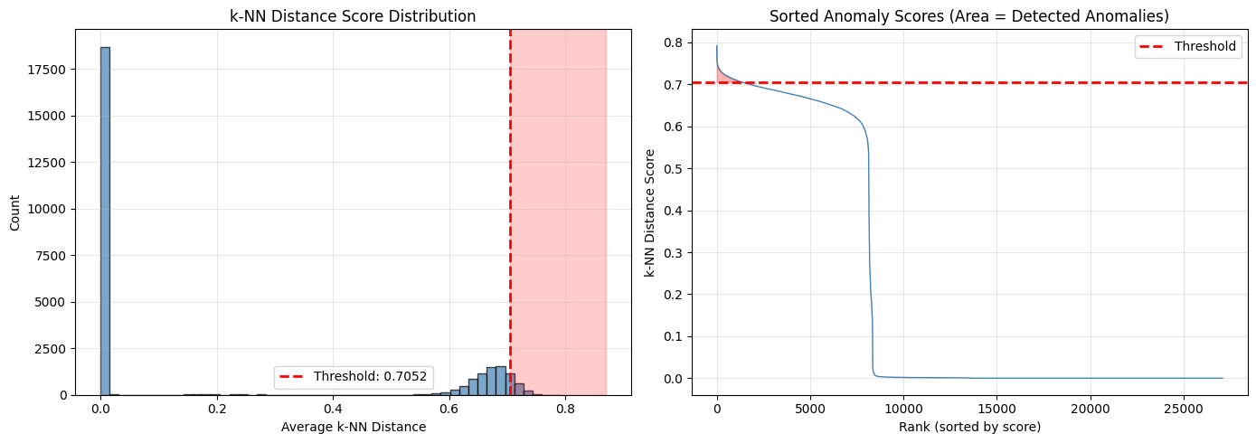
Interpretation:
- Left plot: Most events cluster at low distance (normal)
- Right tail beyond threshold = anomalies
- If distribution is uniform: embeddings may not capture anomaly patterns
How to read these k-NN score charts
Left (Score histogram):
Most events should cluster at low distances (the tall bars on the left)
The red dashed line is the threshold - events beyond it are flagged as anomalies
The red shaded area shows the “anomaly zone”
A long tail suggests good separation between normal and anomalous events
Right (Sorted scores):
Events sorted from highest to lowest anomaly score
The steep initial drop = clear anomalies (high scores)
The red filled area = detected anomalies
A gradual curve suggests ambiguous boundary between normal and anomalous
3. Local Outlier Factor (LOF)
Idea: Anomalies are in regions of lower density than their neighbors.
LOF compares the local density of a point to its neighbors:
LOF ≈ 1: Similar density to neighbors (normal)
LOF > 1: Lower density than neighbors (anomaly)
Advantage over k-NN distance: LOF adapts to varying local densities. A point can be far from the main cluster but still normal if its local area has similar density.
What you should expect:
LOF scores centered around 1 for normal events
Anomalies have LOF > 1 (often > 1.5)
def detect_anomalies_lof(embeddings, n_neighbors=20, contamination=0.05):
    """
    Detect anomalies using Local Outlier Factor.

    Args:
        embeddings: (N, d) array of embeddings
        n_neighbors: Number of neighbors for density estimation
        contamination: Expected anomaly proportion

    Returns:
        predictions: 1 for anomaly, 0 for normal
        scores: Outlier factor (higher = more anomalous)
    """
    lof = LocalOutlierFactor(n_neighbors=n_neighbors, contamination=contamination)
    lof_predictions = lof.fit_predict(embeddings)

    # Convert: LOF returns -1 for anomalies, 1 for normal
    predictions = (lof_predictions == -1).astype(int)

    # Scores (negative_outlier_factor_ is more negative for anomalies)
    # Flip so higher = more anomalous
    scores = -lof.negative_outlier_factor_

    return predictions, scores

# Run LOF detection
lof_preds, lof_scores = detect_anomalies_lof(embeddings, n_neighbors=20, contamination=0.05)

print("Local Outlier Factor (LOF) Detection Results:")
print(f"  n_neighbors: 20")
print(f"  Contamination: 5%")
print(f"  Anomalies detected: {lof_preds.sum()} ({lof_preds.mean():.2%})")
print(f"\nLOF Score Statistics:")
print(f"  Min: {lof_scores.min():.4f} (most normal)")
print(f"  Median: {np.median(lof_scores):.4f}")
print(f"  Max: {lof_scores.max():.4f} (most anomalous)")
Local Outlier Factor (LOF) Detection Results:
n_neighbors: 20
Contamination: 5%
Anomalies detected: 1355 (5.00%)
LOF Score Statistics:
Min: 0.9076 (most normal)
Median: 1.0000
Max: 922272.8750 (most anomalous)
4. Isolation Forest
Idea: Anomalies are easier to “isolate” with random splits.
Build random trees that recursively split data:
Normal points require many splits to isolate (deep in tree)
Anomalies require few splits (shallow in tree)
Advantages:
Very fast (O(n log n) training)
Works well in high dimensions
No distance metric needed
What you should expect:
Scores in [-1, 0] range (sklearn convention)
More negative = more anomalous
def detect_anomalies_isolation_forest(embeddings, contamination=0.05, n_estimators=100):
    """
    Detect anomalies using Isolation Forest.

    Args:
        embeddings: (N, d) array of embeddings
        contamination: Expected anomaly proportion
        n_estimators: Number of trees

    Returns:
        predictions: 1 for anomaly, 0 for normal
        scores: Anomaly score (higher = more anomalous)
    """
    iso = IsolationForest(contamination=contamination, n_estimators=n_estimators, random_state=42)
    iso_predictions = iso.fit_predict(embeddings)

    # Convert: Isolation Forest returns -1 for anomalies, 1 for normal
    predictions = (iso_predictions == -1).astype(int)

    # Scores (score_samples returns negative values, more negative = more anomalous)
    # Flip so higher = more anomalous
    scores = -iso.score_samples(embeddings)

    return predictions, scores

# Run Isolation Forest detection
iso_preds, iso_scores = detect_anomalies_isolation_forest(embeddings, contamination=0.05)

print("Isolation Forest Detection Results:")
print(f"  n_estimators: 100")
print(f"  Contamination: 5%")
print(f"  Anomalies detected: {iso_preds.sum()} ({iso_preds.mean():.2%})")
print(f"\nIsolation Score Statistics:")
print(f"  Min: {iso_scores.min():.4f} (most normal)")
print(f"  Median: {np.median(iso_scores):.4f}")
print(f"  Max: {iso_scores.max():.4f} (most anomalous)")
Isolation Forest Detection Results:
n_estimators: 100
Contamination: 5%
Anomalies detected: 1352 (4.99%)
Isolation Score Statistics:
Min: 0.3919 (most normal)
Median: 0.4585
Max: 0.5428 (most anomalous)
5. Compare Detection Methods
Different methods catch different types of anomalies:
k-NN distance: Global outliers (far from everything)
LOF: Local outliers (normal globally, anomalous locally)
Isolation Forest: Points that are easy to separate
What you should expect:
Methods often agree on obvious anomalies (>80% agreement)
Disagreement on edge cases is normal
If labeled data available, compare precision/recall
# Compare score distributions
fig, axes = plt.subplots(1, 3, figsize=(15, 4))

methods = [
    ('k-NN Distance', knn_scores, knn_preds),
    ('LOF', lof_scores, lof_preds),
    ('Isolation Forest', iso_scores, iso_preds)
]

for ax, (name, scores, preds) in zip(axes, methods):
    # Plot normal vs anomaly score distributions
    normal_scores = scores[preds == 0]
    anomaly_scores = scores[preds == 1]

    ax.hist(normal_scores, bins=30, alpha=0.7, label=f'Normal (n={len(normal_scores)})', color='blue')
    ax.hist(anomaly_scores, bins=30, alpha=0.7, label=f'Anomaly (n={len(anomaly_scores)})', color='red')
    ax.set_xlabel('Anomaly Score')
    ax.set_ylabel('Count')
    ax.set_title(name)
    ax.legend()

plt.tight_layout()
plt.show()

print("Interpretation:")
print("- Good separation between blue (normal) and red (anomaly) = method works well")
print("- Overlap = method is uncertain about those events")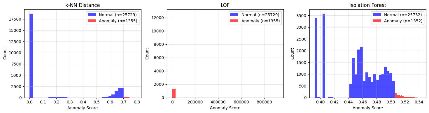
Interpretation:
- Good separation between blue (normal) and red (anomaly) = method works well
- Overlap = method is uncertain about those events
How to read these method comparison charts
Each subplot shows one detection method’s score distribution split by prediction:
Blue: Events classified as normal
Red: Events classified as anomalous
What good separation looks like:
Blue and red distributions have minimal overlap
Red is clearly shifted to higher scores
The boundary between them is sharp
What poor separation looks like:
Blue and red heavily overlap
Hard to distinguish normal from anomalous
Consider different parameters or methods
# Method agreement analysis
print("Method Agreement Analysis:")
print("\nPairwise Agreement (% of events classified the same):")
print(f"  k-NN & LOF:        {(knn_preds == lof_preds).mean():.1%}")
print(f"  k-NN & IsoForest:  {(knn_preds == iso_preds).mean():.1%}")
print(f"  LOF & IsoForest:   {(lof_preds == iso_preds).mean():.1%}")

# Venn-style breakdown
all_agree_anomaly = ((knn_preds == 1) & (lof_preds == 1) & (iso_preds == 1)).sum()
all_agree_normal = ((knn_preds == 0) & (lof_preds == 0) & (iso_preds == 0)).sum()
only_knn = ((knn_preds == 1) & (lof_preds == 0) & (iso_preds == 0)).sum()
only_lof = ((knn_preds == 0) & (lof_preds == 1) & (iso_preds == 0)).sum()
only_iso = ((knn_preds == 0) & (lof_preds == 0) & (iso_preds == 1)).sum()

print(f"\nDetection Breakdown:")
print(f"  All 3 agree (anomaly):  {all_agree_anomaly} events")
print(f"  All 3 agree (normal):   {all_agree_normal} events")
print(f"  Only k-NN detects:      {only_knn} events")
print(f"  Only LOF detects:       {only_lof} events")
print(f"  Only IsoForest detects: {only_iso} events")
Method Agreement Analysis:
Pairwise Agreement (% of events classified the same):
k-NN & LOF: 90.1%
k-NN & IsoForest: 91.5%
LOF & IsoForest: 90.3%
Detection Breakdown:
All 3 agree (anomaly): 9 events
All 3 agree (normal): 23269 events
Only k-NN detects: 1151 events
Only LOF detects: 1307 events
Only IsoForest detects: 1119 events
# Evaluate against labels if available
def evaluate_detector(true_labels, predictions, scores, method_name):
    """Evaluate detection performance."""
    precision = precision_score(true_labels, predictions, zero_division=0)
    recall = recall_score(true_labels, predictions, zero_division=0)
    f1 = f1_score(true_labels, predictions, zero_division=0)

    try:
        auc = roc_auc_score(true_labels, scores)
    except:
        auc = 0.0

    return {
        'Method': method_name,
        'Precision': precision,
        'Recall': recall,
        'F1': f1,
        'AUC': auc
    }

if has_labels:
    print("Evaluating against labeled data...\n")

    n_eval = min(len(eval_df), len(embeddings))

    if 'is_anomaly' in eval_df.columns:
        true_labels = eval_df['is_anomaly'].values[:n_eval]

        results = []
        results.append(evaluate_detector(true_labels, knn_preds[:n_eval], knn_scores[:n_eval], 'k-NN Distance'))
        results.append(evaluate_detector(true_labels, lof_preds[:n_eval], lof_scores[:n_eval], 'LOF'))
        results.append(evaluate_detector(true_labels, iso_preds[:n_eval], iso_scores[:n_eval], 'Isolation Forest'))

        results_df = pd.DataFrame(results)
        print("Method Comparison:")
        print(results_df.to_string(index=False))
        print("\nInterpretation:")
        print("- Precision: % of detected anomalies that are true anomalies")
        print("- Recall: % of true anomalies that were detected")
        print("- F1: Harmonic mean of precision and recall")
        print("- AUC: Overall ranking quality (1.0 = perfect)")
else:
    print("No labels available for evaluation.")
    print("Using method agreement as a proxy for confidence.")
Evaluating against labeled data...
Method Comparison:
Method Precision Recall F1 AUC
k-NN Distance 0.000000 0.000000 0.000000 0.436178
LOF 0.017857 0.071429 0.028571 0.496450
Isolation Forest 0.047619 0.071429 0.057143 0.547341
Interpretation:
- Precision: % of detected anomalies that are true anomalies
- Recall: % of true anomalies that were detected
- F1: Harmonic mean of precision and recall
- AUC: Overall ranking quality (1.0 = perfect)
6. Ensemble Detection
Combine multiple methods for more robust detection.
Strategy: Flag as anomaly if ≥ 2 out of 3 methods agree.
Benefits:
Reduces false positives (need multiple methods to agree)
Catches different anomaly types (each method has strengths)
More reliable for alerting systems
def ensemble_detection(predictions_list, threshold=2):
    """
    Ensemble detection: flag as anomaly if >= threshold methods agree.

    Args:
        predictions_list: List of prediction arrays
        threshold: Minimum votes needed to flag as anomaly

    Returns:
        predictions: 1 for anomaly, 0 for normal
    """
    votes = np.sum(predictions_list, axis=0)
    return (votes >= threshold).astype(int)

# Combine all three methods
ensemble_preds = ensemble_detection([knn_preds, lof_preds, iso_preds], threshold=2)

print("Ensemble Detection (2/3 agreement):")
print(f"  Anomalies detected: {ensemble_preds.sum()} ({ensemble_preds.mean():.2%})")

# Compare to individual methods
print(f"\nComparison:")
print(f"  k-NN alone:      {knn_preds.sum()} anomalies")
print(f"  LOF alone:       {lof_preds.sum()} anomalies")
print(f"  IsoForest alone: {iso_preds.sum()} anomalies")
print(f"  Ensemble (2/3):  {ensemble_preds.sum()} anomalies")
Ensemble Detection (2/3 agreement):
Anomalies detected: 238 (0.88%)
Comparison:
k-NN alone: 1355 anomalies
LOF alone: 1355 anomalies
IsoForest alone: 1352 anomalies
Ensemble (2/3): 238 anomalies
# Visualize ensemble voting
votes = knn_preds + lof_preds + iso_preds

fig, axes = plt.subplots(1, 2, figsize=(14, 5))

# Vote distribution
vote_counts = [np.sum(votes == i) for i in range(4)]
colors = ['green', 'lightgreen', 'orange', 'red']
bars = axes[0].bar(['0 (Normal)', '1 (Maybe)', '2 (Likely)', '3 (Certain)'],
                  vote_counts, color=colors, edgecolor='black')
axes[0].set_xlabel('Number of Methods Flagging as Anomaly')
axes[0].set_ylabel('Number of Events')
axes[0].set_title('Ensemble Vote Distribution')
for bar, count in zip(bars, vote_counts):
    axes[0].text(bar.get_x() + bar.get_width()/2, bar.get_height() + 50,
                str(count), ha='center', va='bottom')

# Score correlation between methods
axes[1].scatter(knn_scores, iso_scores, c=lof_scores, cmap='RdYlGn_r',
               alpha=0.5, s=10)
axes[1].set_xlabel('k-NN Distance Score')
axes[1].set_ylabel('Isolation Forest Score')
axes[1].set_title('Score Correlation (color = LOF score)')
plt.colorbar(axes[1].collections[0], ax=axes[1], label='LOF Score')

plt.tight_layout()
plt.show()

print("Interpretation:")
print("- Events with 3 votes are high-confidence anomalies")
print("- Events with 0 votes are high-confidence normal")
print("- 1-2 votes indicate edge cases or method-specific anomalies")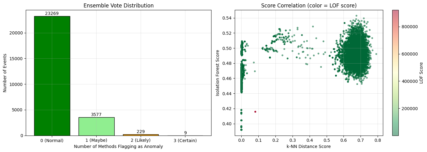
Interpretation:
- Events with 3 votes are high-confidence anomalies
- Events with 0 votes are high-confidence normal
- 1-2 votes indicate edge cases or method-specific anomalies
How to read the ensemble charts
Left (Vote distribution):
Bar heights show how many events received 0, 1, 2, or 3 votes
Green (0 votes): High-confidence normal - no method flagged these
Light green (1 vote): Probably normal, but one method disagrees
Orange (2 votes): Likely anomaly - majority vote
Red (3 votes): High-confidence anomaly - all methods agree
Right (Score correlation):
Each point is an event, positioned by k-NN score (x) and Isolation Forest score (y)
Color indicates LOF score (red = high/anomalous, green = low/normal)
Points in upper-right corner with red color = methods agree on anomaly
Scattered colors = methods disagree
7. Inspect Top Anomalies
Look at the events with highest anomaly scores to understand what the model is catching.
# Load original data for inspection
df = pd.read_parquet('../data/ocsf_logs.parquet')

# Add anomaly scores (match lengths)
df = df.iloc[:len(knn_scores)].copy()
df['knn_score'] = knn_scores[:len(df)]
df['lof_score'] = lof_scores[:len(df)]
df['iso_score'] = iso_scores[:len(df)]
df['ensemble_anomaly'] = ensemble_preds[:len(df)]
df['vote_count'] = votes[:len(df)]

print(f"Added anomaly scores to {len(df)} events.")
Added anomaly scores to 27084 events.
# Top anomalies by ensemble (all 3 methods agree)
high_confidence_anomalies = df[df['vote_count'] == 3].nlargest(10, 'knn_score')

print(f"Top 10 High-Confidence Anomalies (all 3 methods agree):")
print(f"Found {len(df[df['vote_count'] == 3])} total events with 3/3 votes\n")

# Select display columns
display_cols = ['activity_name', 'status', 'actor_user_name', 'http_response_code',
                'knn_score', 'lof_score', 'iso_score']
display_cols = [c for c in display_cols if c in high_confidence_anomalies.columns]

if len(high_confidence_anomalies) > 0:
    high_confidence_anomalies[display_cols].round(4)
else:
    print("No events flagged by all 3 methods.")
Top 10 High-Confidence Anomalies (all 3 methods agree):
Found 9 total events with 3/3 votes
# Analyze what makes these events anomalous
anomalies = df[df['ensemble_anomaly'] == 1]
normals = df[df['ensemble_anomaly'] == 0]

print("Anomaly vs Normal Comparison:")
print("\nActivity Distribution:")
if 'activity_name' in df.columns:
    print("\nAnomalies:")
    print(anomalies['activity_name'].value_counts().head())
    print("\nNormals:")
    print(normals['activity_name'].value_counts().head())

print("\nStatus Distribution:")
if 'status' in df.columns:
    print("\nAnomalies:")
    print(anomalies['status'].value_counts())
    print("\nNormals:")
    print(normals['status'].value_counts())
Anomaly vs Normal Comparison:
Activity Distribution:
Anomalies:
activity_name
Read 230
Create 8
Name: count, dtype: int64
Normals:
activity_name
Read 12884
Unknown 8141
Create 5821
Name: count, dtype: int64
Status Distribution:
Anomalies:
status
Success 238
Name: count, dtype: int64
Normals:
status
Success 26773
Failure 73
Name: count, dtype: int64
8. Save Results
Save anomaly predictions for further analysis or integration with alerting systems.
# Save anomaly predictions
results = pd.DataFrame({
    'knn_score': knn_scores,
    'knn_anomaly': knn_preds,
    'lof_score': lof_scores,
    'lof_anomaly': lof_preds,
    'iso_score': iso_scores,
    'iso_anomaly': iso_preds,
    'ensemble_anomaly': ensemble_preds,
    'vote_count': votes
})

results.to_parquet('../data/anomaly_predictions.parquet')
print(f"Saved anomaly predictions to ../data/anomaly_predictions.parquet")
print(f"  Shape: {results.shape}")
Saved anomaly predictions to ../data/anomaly_predictions.parquet
Shape: (27084, 8)
# Summary statistics
print("\nFinal Summary:")
print("="*50)
print(f"Total events analyzed: {len(embeddings):,}")
print(f"\nDetection Results:")
print(f"  k-NN Distance:     {knn_preds.sum():,} anomalies ({knn_preds.mean():.1%})")
print(f"  LOF:               {lof_preds.sum():,} anomalies ({lof_preds.mean():.1%})")
print(f"  Isolation Forest:  {iso_preds.sum():,} anomalies ({iso_preds.mean():.1%})")
print(f"  Ensemble (2/3):    {ensemble_preds.sum():,} anomalies ({ensemble_preds.mean():.1%})")
print(f"\nConfidence Levels:")
print(f"  High (3/3 votes):  {(votes == 3).sum():,} events")
print(f"  Medium (2/3 votes): {(votes == 2).sum():,} events")
print(f"  Low (1/3 votes):   {(votes == 1).sum():,} events")
print(f"  Normal (0/3 votes): {(votes == 0).sum():,} events")
Final Summary:
==================================================
Total events analyzed: 27,084

Detection Results:
  k-NN Distance:     1,355 anomalies (5.0%)
  LOF:               1,355 anomalies (5.0%)
  Isolation Forest:  1,352 anomalies (5.0%)
  Ensemble (2/3):    238 anomalies (0.9%)

Confidence Levels:
  High (3/3 votes):  9 events
  Medium (2/3 votes): 229 events
  Low (1/3 votes):   3,577 events
  Normal (0/3 votes): 23,269 events
Summary
In this notebook, we:
k-NN Distance: Detected anomalies based on average distance to neighbors
LOF: Used local density comparison for adaptive detection
Isolation Forest: Leveraged tree-based isolation for anomaly scoring
Ensemble: Combined methods for robust detection with voting
Analyzed: Compared methods and inspected top anomalies
Key insights:
Different methods catch different types of anomalies
Ensemble voting (2/3 agreement) reduces false positives
High-confidence anomalies (3/3 votes) deserve immediate attention
LOF adapts to varying local densities (good for multi-modal data)
k-NN distance is simple but effective for global outliers
Production recommendations:
Use ensemble for alerting (fewer false positives)
Use k-NN scores for ranking (continuous severity)
Tune
contaminationbased on your expected anomaly rateConsider using a vector database (FAISS, Milvus) for efficient k-NN at scale
Next steps:
Integrate with alerting system
Set up monitoring for embedding drift
Collect feedback on detected anomalies for model improvement