Part 1: Understanding ResNet Architecture

This tutorial series builds a production-ready anomaly detection system using ResNet embeddings for observability data.

Introduction: Why ResNet for Anomaly Detection?¶

This tutorial explores Residual Networks (ResNet), a breakthrough architecture that enables training of very deep neural networks. While ResNet was originally designed for computer vision, it has emerged as a surprisingly strong baseline for tabular data and embedding models.

Motivation: Tabular Data and Anomaly Detection¶

Recent research has shown that while Transformers (TabTransformer, FT-Transformer) achieve state-of-the-art results on tabular data, ResNet-like architectures provide a simpler, more efficient baseline that often performs comparably well Gorishniy et al. (2021). For applications like:

• Anomaly detection in observability data (logs, network traffic, system metrics)

• Self-supervised learning on unlabelled data

• Creating embeddings for multi-record pattern analysis

ResNet offers several advantages:

1. Simpler architecture than Transformers (no attention mechanism overhead)

2. Linear complexity vs. quadratic attention complexity for high-dimensional tabular data (300+ features)

3. Strong empirical performance on heterogeneous tabular datasets

4. Efficient embedding extraction for downstream clustering and anomaly detection

The Use Case: OCSF Observability Data¶

Consider an observability scenario where you have:

• Unlabelled data: Millions of OCSF (Open Cybersecurity Schema Framework) records

• High dimensionality: 300+ fields per record (categorical and numerical)

• Multi-record anomalies: Patterns that span sequences of events

• No ground truth: Need self-supervised learning

The approach Huang et al. (2020):

1. Pre-train a ResNet to create embeddings from individual records

2. Extract fixed-dimensional vectors that capture “normal” system behavior

3. Detect anomalies as records/sequences that deviate from learned patterns

This tutorial series will build your understanding of ResNet from first principles, then show how to deploy it in production.

Prerequisites¶

Required Background:

• Basic neural network concepts (layers, backpropagation, gradient descent)

• Basic Python and PyTorch syntax

Recommended (but not required):

• Convolutional Neural Networks (CNNs) — This part uses image examples with CNNs, but we include a brief CNN primer before the code

• If you’re primarily interested in tabular data, you can skim the image-based sections and focus on Part 2: Adapting ResNet for Tabular Data

New to neural networks? Start with our Neural Networks From Scratch series:

• NN01: Edge Detection - Understanding neurons as pattern matchers

• NN02: Training from Scratch - Backpropagation and gradient descent

• NN03: General Networks - Building flexible architectures

• NN04: PyTorch Basics - Transitioning to PyTorch (used in this tutorial)

Paper References¶

• Original ResNet: He, K., Zhang, X., Ren, S., & Sun, J. (2016). “Deep Residual Learning for Image Recognition.” CVPR 2016.

• ResNet for Tabular Data: Gorishniy, Y., Rubachev, I., Khrulkov, V., & Babenko, A. (2021). “Revisiting Deep Learning Models for Tabular Data.” NeurIPS 2021.

• TabTransformer Comparison: Huang, X., Khetan, A., Cvitkovic, M., & Karnin, Z. (2020). “TabTransformer: Tabular Data Modeling Using Contextual Embeddings.” arXiv preprint.

The Problem ResNet Solves¶

The Degradation Problem¶

Intuitively, deeper neural networks should be more powerful:

• More layers → More capacity to learn complex patterns

• A 56-layer network should perform at least as well as a 28-layer network (it could just learn identity mappings for the extra layers)

What is an identity mapping? A transformation where the output equals the input: $f(x) = x$. Think of it like a “do nothing” operation - data passes through unchanged. For example, if a layer receives a vector [1, 2, 3], an identity mapping would output exactly [1, 2, 3]. In theory, deeper networks could use identity mappings in extra layers to match shallower networks, but in practice they fail to learn even this simple operation.

But in practice, this doesn’t happen.

import logging
import warnings

logging.getLogger("matplotlib.font_manager").setLevel(logging.ERROR)

import numpy as np
import matplotlib.pyplot as plt

# Simulated training/test error for plain networks
depths = [20, 32, 44, 56]
train_errors_plain = [15.5, 14.2, 15.8, 18.5]
test_errors_plain = [21.3, 20.1, 22.5, 25.7]

# Simulated errors for ResNet
train_errors_resnet = [15.5, 13.8, 12.5, 11.2]
test_errors_resnet = [21.3, 19.5, 18.1, 16.8]

fig, (ax1, ax2) = plt.subplots(1, 2, figsize=(12, 4))

# Plain networks
ax1.plot(depths, train_errors_plain, 'o-', label='Training Error', linewidth=2, markersize=8)
ax1.plot(depths, test_errors_plain, 's-', label='Test Error', linewidth=2, markersize=8)
ax1.set_xlabel('Network Depth (layers)', fontsize=12)
ax1.set_ylabel('Error (%)', fontsize=12)
ax1.set_title('Plain Networks: Degradation Problem', fontsize=13, fontweight='bold')
ax1.legend()
ax1.grid(True, alpha=0.3)
ax1.set_ylim([10, 27])

# ResNets
ax2.plot(depths, train_errors_resnet, 'o-', label='Training Error', linewidth=2, markersize=8, color='green')
ax2.plot(depths, test_errors_resnet, 's-', label='Test Error', linewidth=2, markersize=8, color='darkgreen')
ax2.set_xlabel('Network Depth (layers)', fontsize=12)
ax2.set_ylabel('Error (%)', fontsize=12)
ax2.set_title('Residual Networks: Problem Solved', fontsize=13, fontweight='bold')
ax2.legend()
ax2.grid(True, alpha=0.3)
ax2.set_ylim([10, 27])

plt.tight_layout()
plt.show()

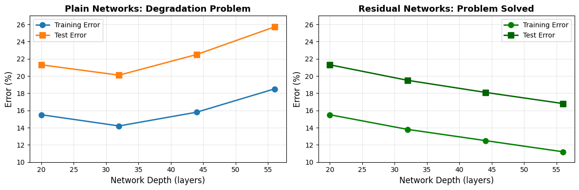
Key Observation: Beyond a certain depth (~20-30 layers), plain networks start to perform worse on both training and test sets. This isn’t overfitting (training error increases too) — it’s optimization difficulty.

Why Plain Networks Fail¶

Two main issues:

1. Vanishing Gradients: As gradients backpropagate through many layers, they get multiplied by small weight matrices repeatedly, shrinking exponentially. Deep layers learn very slowly or not at all.

2. Degraded Optimization Landscape: Very deep networks create complex, non-convex loss surfaces that are hard for SGD to navigate. Even though a solution exists (copy the shallower network and make extra layers just pass data through unchanged), the optimizer can’t find it.

What We Need¶

An architecture where:

• Deeper is easier to optimize, not harder

• Identity mappings are learnable by default

• Gradients flow freely to early layers

This is exactly what ResNet provides.

The Core Innovation — Residual Connections¶

The Residual Block¶

The Key Idea:

In a traditional neural network, layers learn to transform input $\mathbf{x}$ into output $H(\mathbf{x})$ directly:

• Input $\mathbf{x}$ → [layers] → Output $H(\mathbf{x})$

• The layers must learn the complete transformation from scratch

ResNet changes this by learning the residual (the difference between output and input):

Where:

• $\mathbf{x}$: Input to the block

• $F(\mathbf{x})$: Residual — the learned difference/change to apply (typically 2-3 conv/linear layers)

• $H(\mathbf{x})$: Output = Input + Residual change

• $+\mathbf{x}$: The skip connection (also called shortcut connection) — adds input directly to output

Why this helps:

• Instead of learning the full transformation $H(\mathbf{x})$ from scratch, layers only learn what to change ($F(\mathbf{x})$)

• If no change is needed, layers can learn $F(\mathbf{x}) = 0$ (much easier than learning identity)

• The input $\mathbf{x}$ always flows through unchanged via the skip connection

Visual comparison: The diagrams below show the key architectural difference:

• Left (Plain Block): Learns the entire transformation $H(x)$ directly from scratch

• Right (Residual Block): Only learns the residual $F(x)$ to add to the input, where $H(x) = F(x) + x$

Why This Works: Intuition¶

Learning Identity is Easy:

• If the optimal mapping is identity (output = input, i.e., $H(\mathbf{x}) = \mathbf{x}$), the network just needs to learn $F(\mathbf{x}) = 0$

• Why? Because $H(\mathbf{x}) = F(\mathbf{x}) + \mathbf{x}$, so if $H(\mathbf{x}) = \mathbf{x}$, then:

  $$\mathbf{x} = F(\mathbf{x}) + \mathbf{x} \implies F(\mathbf{x}) = 0$$

  (2)

• Pushing weights toward zero is much easier than learning the identity function from scratch with many layers

• This means “doing nothing” (keeping the input unchanged) is easy to learn

Gradient Flow:

• Gradients flow through both paths (main path and skip connection)

• Skip connection provides a “gradient highway” directly to earlier layers

• Even if $F(\mathbf{x})$ has vanishing gradients, $\mathbf{x}$ passes through unchanged

Source

import logging
import warnings

logging.getLogger("matplotlib.font_manager").setLevel(logging.ERROR)

import torch
import torch.nn as nn
import matplotlib.pyplot as plt
import numpy as np

# Simple plain network (no skip connections)
class PlainNetwork(nn.Module):
    def __init__(self, num_layers=10):
        super().__init__()
        self.layers = nn.ModuleList([
            nn.Linear(128, 128) for _ in range(num_layers)
        ])

    def forward(self, x):
        for layer in self.layers:
            x = torch.relu(layer(x))
        return x

# Simple residual network (with skip connections)
class ResidualNetwork(nn.Module):
    def __init__(self, num_layers=10):
        super().__init__()
        self.layers = nn.ModuleList([
            nn.Linear(128, 128) for _ in range(num_layers)
        ])

    def forward(self, x):
        for layer in self.layers:
            x = torch.relu(layer(x)) + x  # Skip connection!
        return x

# Create networks
plain_net = PlainNetwork(num_layers=10)
resnet = ResidualNetwork(num_layers=10)

# Dummy input and target
x = torch.randn(32, 128)
target = torch.randn(32, 128)

# Forward + backward for plain network
plain_output = plain_net(x)
plain_loss = ((plain_output - target) ** 2).mean()
plain_loss.backward()

# Collect gradient magnitudes for each layer
plain_grads = []
for layer in plain_net.layers:
    if layer.weight.grad is not None:
        plain_grads.append(layer.weight.grad.abs().mean().item())

# Reset and do the same for ResNet
resnet.zero_grad()
resnet_output = resnet(x)
resnet_loss = ((resnet_output - target) ** 2).mean()
resnet_loss.backward()

resnet_grads = []
for layer in resnet.layers:
    if layer.weight.grad is not None:
        resnet_grads.append(layer.weight.grad.abs().mean().item())

# Plot comparison
fig, ax = plt.subplots(figsize=(10, 6))

layers = list(range(1, len(plain_grads) + 1))
ax.plot(layers, plain_grads, 'o-', color='red', linewidth=2,
        markersize=8, label='Plain Network')
ax.plot(layers, resnet_grads, 's-', color='blue', linewidth=2,
        markersize=8, label='ResNet (with skip connections)')

ax.set_xlabel('Layer Depth (1 = earliest layer)', fontsize=12, fontweight='bold')
ax.set_ylabel('Gradient Magnitude', fontsize=12, fontweight='bold')
ax.set_title('Gradient Flow Comparison: Plain vs ResNet\n(Lower layers = earlier in network)',
             fontsize=14, fontweight='bold')
ax.legend(fontsize=11)
ax.grid(True, alpha=0.3)
ax.set_yscale('log')  # Log scale to show exponential decay

# Add annotations
ax.annotate('Vanishing gradients\nin plain network',
            xy=(2, plain_grads[1]), xytext=(3, plain_grads[1]*10),
            arrowprops=dict(arrowstyle='->', color='red', lw=1.5),
            fontsize=10, color='red')
ax.annotate('Strong gradients maintained\nvia skip connections',
            xy=(2, resnet_grads[1]), xytext=(5, resnet_grads[1]*0.1),
            arrowprops=dict(arrowstyle='->', color='blue', lw=1.5),
            fontsize=10, color='blue')

plt.tight_layout()
plt.show()

print("Observation:")
print(f"  Plain Network - Layer 1 gradient: {plain_grads[0]:.6f}")
print(f"  Plain Network - Layer 10 gradient: {plain_grads[-1]:.6f}")
print(f"  Ratio (layer 10 / layer 1): {plain_grads[-1] / plain_grads[0]:.6f}")
print()
print(f"  ResNet - Layer 1 gradient: {resnet_grads[0]:.6f}")
print(f"  ResNet - Layer 10 gradient: {resnet_grads[-1]:.6f}")
print(f"  Ratio (layer 10 / layer 1): {resnet_grads[-1] / resnet_grads[0]:.6f}")
print()
print("Key insight: ResNet maintains much stronger gradients in early layers,")
print("enabling effective training of deep networks.")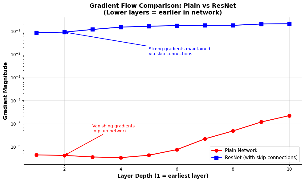

Observation:
  Plain Network - Layer 1 gradient: 0.000000
  Plain Network - Layer 10 gradient: 0.000022
  Ratio (layer 10 / layer 1): 49.664504

  ResNet - Layer 1 gradient: 0.084232
  ResNet - Layer 10 gradient: 0.204147
  Ratio (layer 10 / layer 1): 2.423623

Key insight: ResNet maintains much stronger gradients in early layers,
enabling effective training of deep networks.

What you’re seeing:

• Red line (Plain Network): Gradients decay exponentially as you go to earlier layers (left side of plot)

• Blue line (ResNet): Gradients remain strong throughout all layers due to skip connections

• Log scale: Shows the exponential nature of gradient decay in plain networks

Why this matters for training: Without strong gradients in early layers, those layers barely update during training, making deep plain networks fail to learn effectively. ResNets solve this.

Building Blocks: Basic vs Bottleneck¶

ResNet comes in several standard variants with different depths: ResNet-18, ResNet-34, ResNet-50, ResNet-101, and ResNet-152. The number indicates the total layer count (e.g., ResNet-50 has 50 layers total). These variants use two different types of residual blocks:

• Shallower networks (ResNet-18, ResNet-34) use basic blocks with 2 layers each

• Deeper networks (ResNet-50, ResNet-101, ResNet-152) use bottleneck blocks with 3 layers each for parameter efficiency

Let’s understand the difference between these two block types.

Basic Block (2 Layers)¶

Used in ResNet-18 and ResNet-34. Simple structure with 2 layers:

Architecture: Input → Layer 1 → Layer 2 → Add skip connection → Output

Skip connection: $H(x) = F(x) + x$ where $F(x)$ is computed through 2 layers

When to use: Shallower networks (18-34 layers) where parameter count isn’t a concern

Bottleneck Block (3 Layers)¶

Used in ResNet-50, ResNet-101, and ResNet-152. Optimized structure using reduce-compute-expand:

Architecture: Input → Reduce → Compute → Expand → Add skip connection → Output

The pattern:

1. Reduce dimensions (e.g., $256 \rightarrow 64$ features) - cheap, small transformation

2. Compute on reduced dimensions - expensive operations, but on fewer features

3. Expand back to original size (e.g., $64 \rightarrow 256$ features) - cheap, small transformation

Parameter savings: For 256-dimensional features:

• Basic block (2 layers): ~589,824 parameters

• Bottleneck block (3 layers): ~69,632 parameters (88% reduction!)

When to use: Deeper networks (50+ layers) where parameter efficiency is critical

Why This Works: Intuition¶

The bottleneck design is based on a key insight: most of the useful computation can happen in a lower-dimensional space.

Analogy: Think of data compression. A high-resolution image can be compressed to a smaller size, processed efficiently, then decompressed back. The compressed version still captures the essential information needed for processing.

What’s happening:

1. Reduce (1×1 conv/linear): Projects high-dimensional features into a compact representation that captures the essential patterns. Like compressing an image before editing it.

2. Compute (3×3 conv/linear): Performs the expensive transformations on this compact representation. Since we’re working with fewer dimensions (64 instead of 256), this is much cheaper.

3. Expand (1×1 conv/linear): Projects back to the original high-dimensional space. Like decompressing after processing.

Why it doesn’t hurt performance: The network learns to project into a lower-dimensional subspace where the meaningful transformations happen. The high dimensionality at input/output provides representational capacity, but the actual computation happens efficiently in the bottleneck.

Concrete example (256-dim features):

• Basic block: Two 256×256 transformations = 2 × (256² = 65,536) = ~131K params (plus bias/batch norm)

• Bottleneck block: 256×64 + 64×64 + 64×256 = 16,384 + 4,096 + 16,384 = ~37K params (88% reduction!)

The bottleneck achieves similar representational power with far fewer parameters by concentrating computation in a lower-dimensional space.

Visual Comparison¶

Basic Block (2 layers):

Bottleneck Block (3 layers):

Diagram explanation:

• Both blocks use skip connections (dotted arrows) - the core ResNet innovation

• Basic block: Direct 256→256 transformations (more parameters)

• Bottleneck block: 256→64→64→256 (fewer parameters - processes in narrow 64-dim space)

ResNet Architecture Overview¶

A full ResNet stacks these blocks into a multi-stage architecture:

Architecture components:

1. Initial feature extraction: Transform raw input into initial feature representation

2. Residual stages: Groups of residual blocks, typically 4 stages with increasing feature dimensions (64→128→256→512)

3. Aggregation: Pool/reduce features to fixed size

4. Output head: Final layer(s) for the task (classification, embedding, etc.)

Standard architectures:

• ResNet-18: [2, 2, 2, 2] basic blocks per stage = 18 layers total

• ResNet-34: [3, 4, 6, 3] basic blocks per stage = 34 layers total

• ResNet-50: [3, 4, 6, 3] bottleneck blocks per stage = 50 layers total

• ResNet-101: [3, 4, 23, 3] bottleneck blocks per stage = 101 layers total

• ResNet-152: [3, 8, 36, 3] bottleneck blocks per stage = 152 layers total

Key pattern: Each stage typically:

• Increases feature dimensions (64 → 128 → 256 → 512)

• Maintains or reduces spatial/record dimensions

• Contains multiple residual blocks stacked together

Why this works: The deep stack of residual stages allows the network to learn increasingly abstract representations (from simple patterns to complex concepts), while skip connections ensure gradient flow to all layers.

Summary¶

In this part, you learned the core concepts behind Residual Networks:

1. The degradation problem: Why plain deep networks fail to train effectively

2. Residual connections ($H(x) = F(x) + x$): The skip connection that solves the problem

3. Why it works:

   • Makes learning identity mappings easy ($F(x) = 0$)

   • Enables gradient flow through skip connections (the “gradient highway”)

   • Empirically verified with gradient magnitude visualization

4. Architecture patterns:

   • Basic blocks (2 layers) for shallower networks (ResNet-18/34)

   • Bottleneck blocks (3 layers) for deeper networks (ResNet-50+)

   • Multi-stage design with increasing feature dimensions

Key takeaway: The skip connection is a simple but powerful innovation that makes deep networks trainable. The concept works across all domains—images, text, tabular data—making ResNet one of the most versatile architectures in deep learning.

Next: In Part 2: TabularResNet, you’ll see how to apply these concepts to tabular OCSF data using Linear layers instead of convolutions, plus categorical embeddings for high-cardinality features.

References¶

References

- Gorishniy, Y., Rubachev, I., Khrulkov, V., & Babenko, A. (2021). Revisiting Deep Learning Models for Tabular Data. Advances in Neural Information Processing Systems (NeurIPS), 34, 18932–18943.
- Huang, X., Khetan, A., Cvitkovic, M., & Karnin, Z. (2020). TabTransformer: Tabular Data Modeling Using Contextual Embeddings. arXiv Preprint arXiv:2012.06678.