Theory: See Part 3: Feature Engineering for OCSF Data for the concepts behind these techniques.
This notebook demonstrates feature engineering techniques for OCSF (Open Cybersecurity Schema Framework) observability data.
What you’ll learn:
Loading and exploring OCSF parquet data
Understanding the schema and available fields
Engineering temporal features
Handling categorical and numerical features
Preparing data for TabularResNet
Prerequisites:
Sample data in
../data/(included in repository)Or generate your own using
../appendix-code/
Why OCSF?
Without OCSF, you would need separate models for each log format:
AWS CloudTrail:
eventSource,eventName,userIdentity.arnOkta:
actor.displayName,outcome.result,target[].typeLinux auditd:
syscall,exe,auid,comm
With OCSF, all sources map to the same schema (class_uid, activity_id, actor.user.name), enabling one embedding model to work across all OCSF-compliant sources.
import pandas as pd
import numpy as np
from datetime import datetime
import matplotlib.pyplot as plt
import warnings
warnings.filterwarnings('ignore')

# Display settings for better DataFrame rendering
pd.set_option('display.max_columns', 50)
pd.set_option('display.max_colwidth', 100)
pd.set_option('display.width', None)
1. Load OCSF Data
The sample data is in OCSF-compliant parquet format with flattened nested fields.
What you should expect:
Several thousand events (our sample has ~27,000 generated over 3 hours)
59 columns representing OCSF fields
Mix of numerical IDs and string descriptions
If you see errors:
FileNotFoundError: Ensure../data/ocsf_logs.parquetexists. Download from the appendix or generate using../appendix-code/ImportErrorfor pyarrow: Runpip install pyarrow
# Load the OCSF logs
df = pd.read_parquet('../data/ocsf_logs.parquet')

print(f"Dataset Summary:")
print(f"  Total events: {len(df):,}")
print(f"  Columns: {len(df.columns)}")
print(f"  Memory usage: {df.memory_usage(deep=True).sum() / 1024**2:.1f} MB")
Dataset Summary:
Total events: 27,084
Columns: 59
Memory usage: 84.8 MB
# Preview the data
df.head(3)2. Explore OCSF Schema
OCSF events have a hierarchical structure that has been flattened:
Core fields:
class_uid,category_uid,activity_id,severity_id,timeNested objects:
actor,src_endpoint,dst_endpoint,http_request,http_responseFlattened fields:
actor_user_name,http_request_method, etc.
What you should expect:
Mix of
int64,float64, andobject(string) columnsMany columns may be sparse (lots of nulls) since OCSF fields are optional
Column names follow OCSF naming conventions with underscores
# Data type distribution
dtype_counts = df.dtypes.value_counts()
print("Column types:")
for dtype, count in dtype_counts.items():
    print(f"  {dtype}: {count} columns")

# Visualize column types
fig, ax = plt.subplots(figsize=(8, 4))
dtype_counts.plot(kind='barh', ax=ax, color='steelblue', edgecolor='black')
ax.set_xlabel('Number of Columns')
ax.set_ylabel('Data Type')
ax.set_title('OCSF Column Types')
for i, v in enumerate(dtype_counts):
    ax.text(v + 0.5, i, str(v), va='center')
plt.tight_layout()
plt.show()
Column types:
object: 47 columns
int64: 7 columns
float64: 5 columns
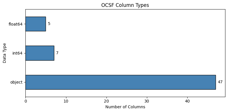
How to read this chart
Shows how many columns are each data type
object= strings (categorical text like “Success”, “GET”)int64/float64= numbers (IDs, timestamps, durations)More object columns = more categorical features to embed
# Key categorical columns and their distributions
categorical_cols = ['class_name', 'category_name', 'activity_name', 'status', 'level', 'service']
categorical_cols = [c for c in categorical_cols if c in df.columns]

fig, axes = plt.subplots(2, 3, figsize=(15, 8))
axes = axes.flatten()

for i, col in enumerate(categorical_cols[:6]):
    value_counts = df[col].value_counts().head(10)
    value_counts.plot(kind='barh', ax=axes[i], color='steelblue', edgecolor='black')
    axes[i].set_title(f'{col} ({df[col].nunique()} unique)')
    axes[i].set_xlabel('Count')

plt.suptitle('Key Categorical Column Distributions', fontsize=14, y=1.02)
plt.tight_layout()
plt.show()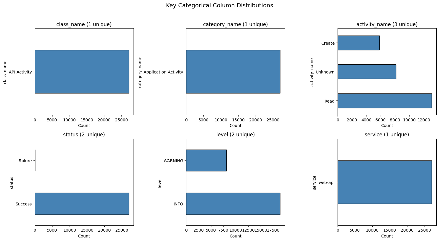
How to read these charts
Each chart shows value counts for a key OCSF field
Bar length = how many events have that value
(N unique)in title = cardinality (vocabulary size for embedding)Single bar (1 unique): Feature is constant - provides no signal for distinguishing events
Highly skewed distributions (one dominant value) provide less signal
Uniform distributions provide more discriminative power
3. Engineer Temporal Features
Time-based patterns are critical for anomaly detection:
Logins at 3 AM are suspicious
Anomaly patterns have timing signatures
Business hours vs off-hours traffic differs significantly
What you should expect:
hour_of_day: 0-23 (midnight = 0)day_of_week: 0-6 (Monday = 0, Sunday = 6)hour_sin/hour_cos: Values between -1 and 1 (cyclical encoding)
Why cyclical encoding? Without it, hour 23 and hour 0 appear far apart (23 vs 0), but they’re actually adjacent times. Sin/cos encoding preserves this circular relationship.
def extract_temporal_features(df, time_col='time'):
    """
    Extract temporal features from Unix timestamp (milliseconds).

    Returns DataFrame with new temporal columns.
    """
    result = df.copy()

    # Convert milliseconds to datetime
    result['datetime'] = pd.to_datetime(result[time_col], unit='ms', errors='coerce')

    # Basic temporal features
    result['hour_of_day'] = result['datetime'].dt.hour
    result['day_of_week'] = result['datetime'].dt.dayofweek  # 0=Monday
    result['is_weekend'] = (result['day_of_week'] >= 5).astype(int)
    result['is_business_hours'] = ((result['hour_of_day'] >= 9) &
                                    (result['hour_of_day'] < 17)).astype(int)

    # Cyclical encoding (sin/cos) - preserves circular nature
    result['hour_sin'] = np.sin(2 * np.pi * result['hour_of_day'] / 24)
    result['hour_cos'] = np.cos(2 * np.pi * result['hour_of_day'] / 24)
    result['day_sin'] = np.sin(2 * np.pi * result['day_of_week'] / 7)
    result['day_cos'] = np.cos(2 * np.pi * result['day_of_week'] / 7)

    return result

# Apply temporal feature extraction
df = extract_temporal_features(df)

# Show sample of temporal features
temporal_cols = ['datetime', 'hour_of_day', 'day_of_week', 'is_weekend',
                 'is_business_hours', 'hour_sin', 'hour_cos']
df[temporal_cols].head()# Visualize temporal distributions
fig, axes = plt.subplots(2, 2, figsize=(14, 10))
# Hour distribution
df['hour_of_day'].hist(bins=24, ax=axes[0, 0], edgecolor='black', color='steelblue')
axes[0, 0].set_xlabel('Hour of Day')
axes[0, 0].set_ylabel('Count')
axes[0, 0].set_title('Event Distribution by Hour')
axes[0, 0].set_xticks(range(0, 24, 2))
# Day of week distribution
day_names = ['Mon', 'Tue', 'Wed', 'Thu', 'Fri', 'Sat', 'Sun']
day_counts = df['day_of_week'].value_counts().sort_index()
axes[0, 1].bar(day_names, [day_counts.get(i, 0) for i in range(7)],
edgecolor='black', color='steelblue')
axes[0, 1].set_xlabel('Day of Week')
axes[0, 1].set_ylabel('Count')
axes[0, 1].set_title('Event Distribution by Day')
# Cyclical encoding visualization
hours = np.arange(24)
hour_sin = np.sin(2 * np.pi * hours / 24)
hour_cos = np.cos(2 * np.pi * hours / 24)
axes[1, 0].plot(hours, hour_sin, 'b-', label='sin(hour)', linewidth=2)
axes[1, 0].plot(hours, hour_cos, 'r-', label='cos(hour)', linewidth=2)
axes[1, 0].set_xlabel('Hour of Day')
axes[1, 0].set_ylabel('Encoded Value')
axes[1, 0].set_title('Cyclical Hour Encoding')
axes[1, 0].legend()
axes[1, 0].set_xticks(range(0, 24, 4))
axes[1, 0].axhline(0, color='gray', linestyle='--', alpha=0.5)
# Show why cyclical encoding matters
axes[1, 1].scatter(hour_sin, hour_cos, c=hours, cmap='hsv', s=100)
for i in [0, 6, 12, 18, 23]:
axes[1, 1].annotate(f'{i}h', (hour_sin[i], hour_cos[i]),
textcoords="offset points", xytext=(5, 5))
axes[1, 1].set_xlabel('hour_sin')
axes[1, 1].set_ylabel('hour_cos')
axes[1, 1].set_title('Hours in (sin, cos) Space\n(Note: 23h and 0h are adjacent!)')
axes[1, 1].set_aspect('equal')
plt.tight_layout()
plt.show()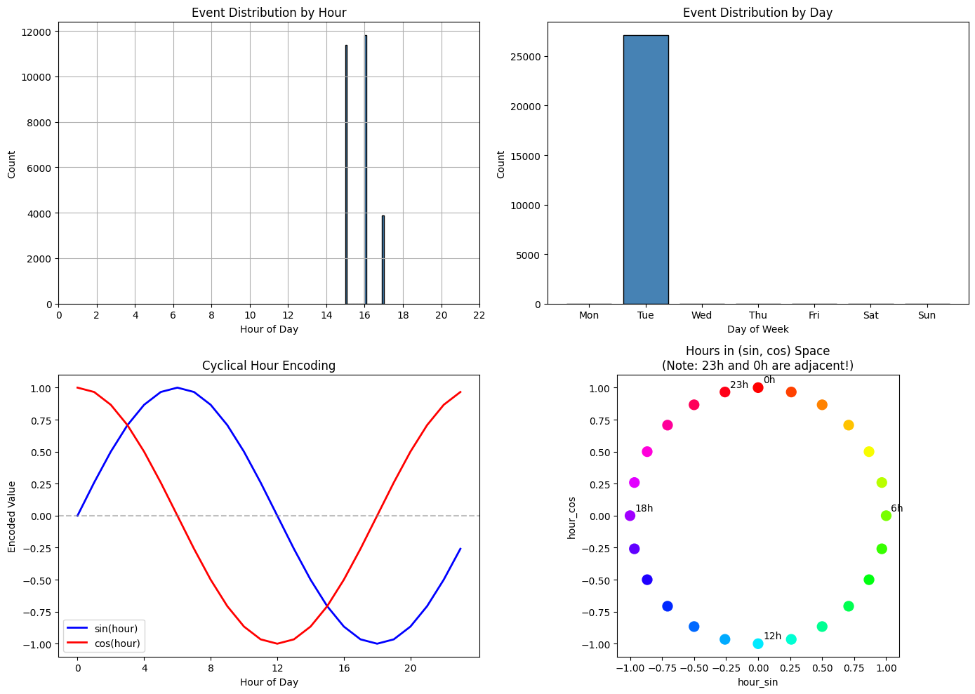
How to read these charts
Top row - Event distributions:
Left (Hour): Shows when events occurred. Spikes indicate hours with more activity. In production data, you’d expect events spread across hours with patterns (e.g., more during business hours).
Right (Day): Shows which days events occurred. Multiple bars indicate events spanning multiple days.
Bottom row - Cyclical encoding explained:
Left (sin/cos curves): Shows how hours map to sin/cos values. Notice that hour 0 and hour 23 have similar values - this is intentional! It captures that midnight and 11 PM are temporally close.
Right (circular plot): Each dot is an hour plotted as (sin, cos) coordinates. Hours form a circle, so 23h and 0h are adjacent - unlike raw hour values where they’d be 23 units apart.
Note on sample data: The synthetic dataset was generated over a 3-hour period. In production OCSF data collected over days/weeks, you’d see realistic temporal distributions where time-of-day patterns become powerful anomaly signals.
4. Select Core Features
Not all 60+ columns are useful for embedding. We select:
Categorical: class, activity, status, severity, user, HTTP method, URL path, response code
Numerical: duration, temporal features (including cyclical encodings)
Categorical vs Numerical decision criteria:
Categorical: Discrete codes/IDs where numerical distance is meaningless
http_response_code: 200, 404, 500 are status classes, not quantitiesseverity_id,activity_id,status_id: OCSF ID codes, not continuous values
Numerical: Continuous values or derived features where math makes sense
duration: Actual time measurementis_weekend,is_business_hours: Binary flags (0/1 works fine)hour_sin,hour_cos: Continuous cyclical encodings
What you should expect:
12 categorical features with varying cardinalities
8 numerical features (duration + temporal)
# Define feature sets
#
# Categorical: Discrete codes/IDs where numerical distance is meaningless
# - http_response_code: 200, 404, 500 are status classes
# - severity_id, activity_id, status_id: OCSF ID codes (not continuous values)
#
# Numerical: Continuous values where arithmetic makes sense
# - duration: actual time measurement
# - Binary flags and cyclical encodings work fine as numeric

categorical_features = [
    'class_name',
    'activity_name',
    'status',
    'level',
    'service',
    'actor_user_name',
    'http_request_method',
    'http_request_url_path',
    'http_response_code',   # Discrete status classes (200, 404, 500)
    'severity_id',          # OCSF severity levels (1=Info, 2=Low, 3=Medium, etc.)
    'activity_id',          # OCSF activity type codes
    'status_id',            # OCSF status codes (0=Unknown, 1=Success, 2=Failure)
]

numerical_features = [
    'duration',             # Continuous: actual time measurement
    'hour_of_day',          # Used for cyclical encoding
    'day_of_week',          # Used for cyclical encoding
    'is_weekend',           # Binary flag (0/1)
    'is_business_hours',    # Binary flag (0/1)
    'hour_sin',             # Continuous cyclical encoding
    'hour_cos',             # Continuous cyclical encoding
    'day_sin',              # Continuous cyclical encoding
    'day_cos',              # Continuous cyclical encoding
]

# Filter to columns that exist in our data
categorical_features = [c for c in categorical_features if c in df.columns]
numerical_features = [c for c in numerical_features if c in df.columns]

print(f"Selected Features:")
print(f"\nCategorical ({len(categorical_features)}):")
for col in categorical_features:
    print(f"  - {col}: {df[col].nunique()} unique values")

print(f"\nNumerical ({len(numerical_features)}):")
for col in numerical_features:
    print(f"  - {col}: range [{df[col].min():.1f}, {df[col].max():.1f}]")
Selected Features:
Categorical (12):
- class_name: 1 unique values
- activity_name: 3 unique values
- status: 2 unique values
- level: 2 unique values
- service: 1 unique values
- actor_user_name: 5 unique values
- http_request_method: 2 unique values
- http_request_url_path: 2279 unique values
- http_response_code: 2 unique values
- severity_id: 3 unique values
- activity_id: 2 unique values
- status_id: 2 unique values
Numerical (9):
- duration: range [0.1, 5000.5]
- hour_of_day: range [15.0, 17.0]
- day_of_week: range [1.0, 1.0]
- is_weekend: range [0.0, 0.0]
- is_business_hours: range [0.0, 1.0]
- hour_sin: range [-1.0, -0.7]
- hour_cos: range [-0.7, -0.3]
- day_sin: range [0.8, 0.8]
- day_cos: range [0.6, 0.6]
5. Handle Missing Values
OCSF events have optional fields. Our strategy:
Categorical: Use special ‘MISSING’ category
Numerical: Use 0 (or median for important features)
What you should expect:
After handling, no nulls should remain
Some categorical columns may show ‘MISSING’ as a frequent value
If you still see nulls:
Check if new columns were added after the missing value handling
Ensure the column list matches what’s in the DataFrame
# Check missing values before handling
all_features = categorical_features + numerical_features
missing_before = df[all_features].isnull().sum()
missing_before = missing_before[missing_before > 0]

if len(missing_before) > 0:
    print("Missing values BEFORE handling:")
    print(missing_before.to_frame('null_count'))
else:
    print("No missing values in selected features.")
Missing values BEFORE handling:
null_count
actor_user_name 8141
http_request_method 8141
http_request_url_path 8141
http_response_code 8141
duration 8141
def handle_missing_values(df, categorical_cols, numerical_cols):
    """
    Handle missing values in feature columns.
    """
    result = df.copy()

    # Categorical: fill with 'MISSING' and convert to string
    # This handles numeric columns like http_response_code correctly
    for col in categorical_cols:
        if col in result.columns:
            # Convert to string first (handles numeric categoricals like http_response_code)
            result[col] = result[col].astype(str)
            result[col] = result[col].replace('nan', 'MISSING').replace('', 'MISSING')

    # Numerical: fill with 0
    for col in numerical_cols:
        if col in result.columns:
            result[col] = pd.to_numeric(result[col], errors='coerce').fillna(0)

    return result

# Apply missing value handling
df_clean = handle_missing_values(df, categorical_features, numerical_features)

# Verify no nulls remain
null_counts = df_clean[all_features].isnull().sum()
if null_counts.sum() > 0:
    print("WARNING: Nulls remaining after handling:")
    print(null_counts[null_counts > 0])
else:
    print("Success: No nulls remaining in feature columns.")
Success: No nulls remaining in feature columns.
6. Encode Features for TabularResNet
TabularResNet needs:
Numerical array: Normalized floats (mean=0, std=1)
Categorical array: Integer indices (0, 1, 2, ...)
What you should expect:
Numerical values centered around 0 with std close to 1
Categorical values as non-negative integers
Cardinalities = vocabulary size + 1 (for UNKNOWN)
If you see unexpected values:
Very large numerical values: Check if outliers need handling
Negative categorical values: Should not happen with LabelEncoder
from sklearn.preprocessing import StandardScaler, LabelEncoder

def prepare_for_tabular_resnet(df, categorical_cols, numerical_cols):
    """
    Prepare features for TabularResNet.

    Returns:
        numerical_array: Normalized numerical features
        categorical_array: Integer-encoded categorical features
        encoders: Dict of LabelEncoders
        scaler: StandardScaler
        cardinalities: List of vocab sizes per categorical
    """
    # Encode categorical features
    encoders = {}
    categorical_data = []
    cardinalities = []

    for col in categorical_cols:
        encoder = LabelEncoder()
        # Add 'UNKNOWN' for handling new values at inference
        unique_vals = list(df[col].unique()) + ['UNKNOWN']
        encoder.fit(unique_vals)
        encoded = encoder.transform(df[col])
        categorical_data.append(encoded)
        encoders[col] = encoder
        cardinalities.append(len(encoder.classes_))

    categorical_array = np.column_stack(categorical_data) if categorical_data else np.array([])

    # Scale numerical features
    scaler = StandardScaler()
    numerical_array = scaler.fit_transform(df[numerical_cols])

    return numerical_array, categorical_array, encoders, scaler, cardinalities

# Prepare features
numerical_array, categorical_array, encoders, scaler, cardinalities = \
    prepare_for_tabular_resnet(df_clean, categorical_features, numerical_features)

print("Feature Arrays Ready for TabularResNet:")
print(f"  Numerical shape: {numerical_array.shape}")
print(f"  Categorical shape: {categorical_array.shape}")
print(f"\nCategorical Cardinalities (vocab size + UNKNOWN):")
for col, card in zip(categorical_features, cardinalities):
    print(f"  {col}: {card}")
Feature Arrays Ready for TabularResNet:
Numerical shape: (27084, 9)
Categorical shape: (27084, 12)
Categorical Cardinalities (vocab size + UNKNOWN):
class_name: 2
activity_name: 4
status: 3
level: 3
service: 2
actor_user_name: 7
http_request_method: 4
http_request_url_path: 2281
http_response_code: 4
severity_id: 4
activity_id: 3
status_id: 3
# Preview numerical features (normalized)
print("Numerical features (first 5 rows, normalized):")
print("Expected: values centered around 0, mostly between -3 and 3")
print()
pd.DataFrame(numerical_array[:5], columns=numerical_features).round(3)
Numerical features (first 5 rows, normalized):
Expected: values centered around 0, mostly between -3 and 3
# Preview categorical features (integer encoded)
print("Categorical features (first 5 rows, integer encoded):")
print("Expected: non-negative integers (0 to cardinality-1)")
print()
pd.DataFrame(categorical_array[:5], columns=categorical_features)
Categorical features (first 5 rows, integer encoded):
Expected: non-negative integers (0 to cardinality-1)
# Visualize numerical feature distributions after scaling
fig, axes = plt.subplots(2, 4, figsize=(16, 8))
axes = axes.flatten()

for i, (col, ax) in enumerate(zip(numerical_features[:8], axes)):
    ax.hist(numerical_array[:, i], bins=50, edgecolor='black', alpha=0.7)
    ax.axvline(0, color='red', linestyle='--', label='mean=0')
    ax.set_title(col)
    ax.set_xlabel('Normalized Value')

plt.suptitle('Numerical Feature Distributions (After StandardScaler)', fontsize=14, y=1.02)
plt.tight_layout()
plt.show()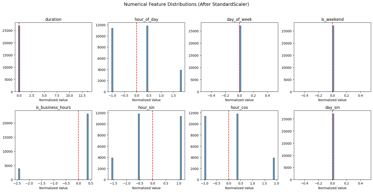
How to read these distributions
Each histogram shows a normalized numerical feature (mean=0 after StandardScaler):
Single spike at 0: Feature has no variance in this dataset. Won’t help with anomaly detection.
Spread distribution: Feature has useful variance. Values far from 0 (beyond ±2) are statistical outliers.
The red dashed line marks mean=0 (the center after normalization).
For this synthetic dataset: Temporal features may show limited variance since events were generated over a 3-hour period. In production data collected over longer periods, you’d see more spread in temporal features.
7. Verify Encoding Quality
Before saving, let’s verify the encoding is correct.
# Verify scaler statistics
print("Scaler Statistics (should show diverse ranges before scaling):")
print()
scaler_stats = pd.DataFrame({
    'feature': numerical_features,
    'original_mean': scaler.mean_,
    'original_std': scaler.scale_
}).round(4)
scaler_stats
Scaler Statistics (should show diverse ranges before scaling):
How to interpret scaler statistics
original_mean: The average value before scaling. Diverse means = features have different scales.
original_std: The standard deviation before scaling.
std ≈ 0means the feature has very low variance - won’t help distinguish eventsstd >> meanmeans high variance (likeduration)
Warning signs:
If many features show very low
std, they won’t help distinguish events (no information)Very large means/stds may indicate outliers that could dominate training
Why duration has std >> mean: This is expected for timing data. Latency/duration features follow long-tailed distributions—most requests complete quickly (small values), but a few take much longer (large outliers). This creates high standard deviation relative to the mean. After scaling, those slow requests become statistical outliers, which is exactly what anomaly detection should flag.
In this output: With data generated over a 3-hour period, you’ll see some variance in temporal features, though production data collected over longer periods would show even more temporal variation.
# Verify categorical encoding can handle UNKNOWN values
print("Testing UNKNOWN handling for categorical encoders:")
print()
for col, encoder in encoders.items():
    # Check UNKNOWN is in classes
    has_unknown = 'UNKNOWN' in encoder.classes_
    unknown_idx = encoder.transform(['UNKNOWN'])[0] if has_unknown else None
    print(f"  {col}: UNKNOWN index = {unknown_idx}")
Testing UNKNOWN handling for categorical encoders:
class_name: UNKNOWN index = 1
activity_name: UNKNOWN index = 2
status: UNKNOWN index = 2
level: UNKNOWN index = 1
service: UNKNOWN index = 0
actor_user_name: UNKNOWN index = 1
http_request_method: UNKNOWN index = 3
http_request_url_path: UNKNOWN index = 2280
http_response_code: UNKNOWN index = 3
severity_id: UNKNOWN index = 3
activity_id: UNKNOWN index = 2
status_id: UNKNOWN index = 2
How to interpret UNKNOWN indices
Each encoder maps category strings to integers. The UNKNOWN index shows where unseen categories will be mapped at inference time.
What to check:
Every encoder should have an UNKNOWN index (not
None)High indices (like
http_request_url_path: 966) indicate high-cardinality features with many unique valuesLow indices indicate low-cardinality features
Why this matters: When new data contains a category not seen during training (e.g., a new user), the pipeline maps it to UNKNOWN rather than crashing. The model learns a generic embedding for “unknown” values.
8. Save Processed Features
Save the processed data and encoding artifacts for training.
Why save these artifacts?
Feature arrays: The training notebook needs preprocessed numerical/categorical arrays, not raw OCSF data
Encoders: At inference time, we must encode new data exactly the same way (same category→integer mappings)
Scaler: New numerical data must be scaled using the training mean/std, not recomputed
Cardinalities: The model architecture depends on vocabulary sizes - must match at load time
Without these artifacts, you’d get mismatched encodings (category “Success” → different integers) or scaling drift.
Files saved:
numerical_features.npy: Normalized numerical featurescategorical_features.npy: Integer-encoded categorical featuresfeature_artifacts.pkl: Encoders, scaler, column names, cardinalities
import pickle

# Save feature arrays
np.save('../data/numerical_features.npy', numerical_array)
np.save('../data/categorical_features.npy', categorical_array)

# Save encoders and scaler
artifacts = {
    'encoders': encoders,
    'scaler': scaler,
    'categorical_cols': categorical_features,
    'numerical_cols': numerical_features,
    'cardinalities': cardinalities
}

with open('../data/feature_artifacts.pkl', 'wb') as f:
    pickle.dump(artifacts, f)

print("Saved files:")
print(f"  - numerical_features.npy: {numerical_array.shape}")
print(f"  - categorical_features.npy: {categorical_array.shape}")
print(f"  - feature_artifacts.pkl: encoders + scaler + metadata")
Saved files:
- numerical_features.npy: (27084, 9)
- categorical_features.npy: (27084, 12)
- feature_artifacts.pkl: encoders + scaler + metadata
Summary
In this notebook, we:
Loaded OCSF data from parquet format (~27,000 events)
Explored the schema - 59 columns with nested objects flattened
Engineered temporal features - hour, day, cyclical sin/cos encoding
Selected core features - 12 categorical + 9 numerical
Handled missing values - ‘MISSING’ for categorical, 0 for numerical
Encoded for TabularResNet - LabelEncoder + StandardScaler
Design decision: OCSF ID fields are treated as categorical:
http_response_code,severity_id,activity_id,status_idare discrete codesEmbedding layers learn semantic relationships between codes
Only truly continuous values (duration, cyclical encodings) are numerical
Key outputs:
Numerical array:
(N, num_features)normalized floatsCategorical array:
(N, cat_features)integer indicesArtifacts: Encoders and scaler for inference
Next: Use these features in 04