Apply various anomaly detection algorithms to your validated embeddings for OCSF observability data.
What you’ll learn: How to detect anomalies using vector DB only - no separate detection model required. The vector database stores embeddings and finds similar records, while different scoring algorithms (distance-based, density-based, etc.) compute anomaly scores from those similarities. All methods work directly on TabularResNet embeddings without training additional models.
Optional extension: Section 6 covers LSTM-based sequence detection for advanced use cases like multi-step anomalies (e.g., cascading failures) - this requires training a separate model and is outside the core vector DB architecture.
Key Terminology
Before diving into detection methods, let’s define the key concepts:
Vector Database: A specialized database optimized for storing embeddings and finding similar vectors quickly using approximate nearest neighbor (ANN) search.
k-NN (k-Nearest Neighbors): Finds the k most similar embeddings to a query embedding. For example, k=20 finds the 20 most similar historical events.
LOF (Local Outlier Factor): Measures how isolated a point is compared to its local neighborhood. Points in sparse regions have high LOF scores (likely anomalies).
Isolation Forest: An algorithm that isolates anomalies by building decision trees. Anomalies are easier to isolate (require fewer splits), so they have shorter path lengths.
Distance metrics:
Cosine similarity: Measures angle between vectors (0=perpendicular, 1=identical direction). Good for when magnitude doesn’t matter.
Euclidean distance: Standard geometric distance. Sensitive to both direction and magnitude.
Negative inner product: Related to cosine but without normalization. Efficient for similarity search.
Contamination: The expected proportion of anomalies in your data (e.g., 0.1 = 10% anomalies). Used to set detection thresholds.
Overview of Anomaly Detection Methods
Once you have high-quality embeddings, you can detect anomalies using a vector database as the central retrieval layer plus multiple scoring algorithms:
Core methods (no additional model training):
Vector DB retrieval: k-NN similarity search for every event
Density-based: Local Outlier Factor (LOF) on neighbor sets
Tree-based: Isolation Forest (optional baseline)
Distance-based: k-NN distance (cosine, Euclidean, negative inner product)
Clustering-based: Distance from cluster centroids
Optional advanced method (requires separate model): 6. Sequence-based: Multi-record anomalies using LSTM (for cascading failures, correlated issues)
Each method has different strengths. We’ll implement all of them and compare.
1. Vector DB Retrieval (Central Layer)
The vector database is the system of record for embeddings. For each incoming event:
Generate the embedding with TabularResNet.
Query the vector DB for k nearest neighbors.
Compute anomaly scores from neighbor distances or density.
Persist the new embedding for future comparisons (if it’s not an outlier).
# Pseudocode interface for a vector DB client
def retrieve_neighbors(vector_db, embedding, k=20):
    """
    Query the vector database for nearest neighbors.

    Returns:
        neighbors: list of (neighbor_id, distance)
    """
    return vector_db.search(embedding, top_k=k)

def score_from_neighbors(neighbors, percentile=95):
    """
    Basic distance-based scoring from neighbor distances.
    """
    distances = [d for _, d in neighbors]
    threshold = np.percentile(distances, percentile)
    score = np.mean(distances)
    return score, threshold

# Example usage
neighbors = retrieve_neighbors(vector_db, embedding, k=20)
score, threshold = score_from_neighbors(neighbors, percentile=95)
is_anomaly = score > threshold
Scaling Notes: FAISS vs Distributed Vector DBs
FAISS is excellent for fast similarity search on a single machine or small clusters, but it is memory-bound and requires careful sharding/replication for very large datasets.
For large-scale, multi-tenant, or high-ingest systems, prefer a distributed vector database with built-in indexing, replication, and all-flash storage.
Example: VAST Data Vector DB for very large volumes and near real-time ingestion.
2. Local Outlier Factor (LOF)
What is LOF? Local Outlier Factor measures how isolated a point is compared to its local neighborhood. Instead of using global distance thresholds, LOF compares each point’s density to its neighbors’ density.
The key insight: An anomaly isn’t just “far away” - it’s in a less dense region than its neighbors. A point can be far from cluster centers but still be normal if its local area has similar density.
How it works:
For each point, find its k nearest neighbors
Compute the local reachability density (how tightly packed the neighborhood is)
Compare this density to the neighbors’ densities
Points in sparser regions get high LOF scores (> 1 = outlier)
When to use LOF:
Multiple clusters with different densities: Common operations might be dense, while rare maintenance tasks are sparser but still normal
Observability data with natural groupings: Different event types (API calls, database queries, background jobs) have different baseline densities
Detecting isolated anomalies: Unusual request patterns that occur in sparse regions, even if not “far” from normal events
Advantages for OCSF observability data:
✅ Adapts to local density (doesn’t penalize naturally sparse event types)
✅ Detects anomalies that hide within legitimate traffic patterns
✅ Works well when anomalies appear in unexpected combinations of features
Disadvantages:
❌ Sensitive to k parameter (too small = noisy, too large = misses local patterns)
❌ Computationally expensive for large datasets (needs k-NN for every point)
❌ Assumes anomalies are isolated (fails if anomalies form dense clusters)
Interpretation:
LOF ≈ 1: Similar density to neighbors (normal)
LOF > 1.5: Significantly less dense than neighbors (likely anomaly)
LOF > 3: Very isolated (strong anomaly signal)
import logging
import warnings

logging.getLogger("matplotlib.font_manager").setLevel(logging.ERROR)

import numpy as np
import matplotlib.pyplot as plt
from sklearn.neighbors import LocalOutlierFactor
from sklearn.metrics import precision_score, recall_score, f1_score, confusion_matrix

def detect_anomalies_lof(embeddings, contamination=0.1, n_neighbors=20):
    """
    Detect anomalies using Local Outlier Factor.

    Args:
        embeddings: (num_samples, embedding_dim) array
        contamination: Expected proportion of anomalies
        n_neighbors: Number of neighbors for density estimation

    Returns:
        predictions: -1 for anomalies, 1 for normal
        scores: Negative outlier factor (more negative = more anomalous)
    """
    lof = LocalOutlierFactor(n_neighbors=n_neighbors, contamination=contamination)
    predictions = lof.fit_predict(embeddings)

    # Negative outlier scores (use negative_outlier_factor_)
    scores = lof.negative_outlier_factor_

    return predictions, scores

# Simulate embeddings with anomalies
np.random.seed(42)

# Normal data: 3 clusters
normal_cluster1 = np.random.randn(200, 256) * 0.5
normal_cluster2 = np.random.randn(200, 256) * 0.5 + 3.0
normal_cluster3 = np.random.randn(200, 256) * 0.5 - 3.0
normal_embeddings = np.vstack([normal_cluster1, normal_cluster2, normal_cluster3])

# Anomalies: scattered outliers
anomaly_embeddings = np.random.uniform(-8, 8, (60, 256))

all_embeddings = np.vstack([normal_embeddings, anomaly_embeddings])
true_labels = np.array([0]*600 + [1]*60)  # 0=normal, 1=anomaly

# Detect anomalies
predictions, scores = detect_anomalies_lof(all_embeddings, contamination=0.1, n_neighbors=20)

# Convert predictions: -1 (anomaly) → 1, 1 (normal) → 0
predicted_labels = (predictions == -1).astype(int)

# Evaluate
precision = precision_score(true_labels, predicted_labels)
recall = recall_score(true_labels, predicted_labels)
f1 = f1_score(true_labels, predicted_labels)

print(f"Local Outlier Factor (LOF) Results:")
print(f"  Precision: {precision:.3f}")
print(f"  Recall:    {recall:.3f}")
print(f"  F1-Score:  {f1:.3f}")
print(f"\nInterpretation:")
print(f"  Precision = {precision:.1%} of flagged items are true anomalies")
print(f"  Recall = {recall:.1%} of true anomalies were detected")
Local Outlier Factor (LOF) Results:
Precision: 0.909
Recall: 1.000
F1-Score: 0.952
Interpretation:
Precision = 90.9% of flagged items are true anomalies
Recall = 100.0% of true anomalies were detected
Visualizing LOF Results
from sklearn.manifold import TSNE

# Reduce to 2D for visualization
tsne = TSNE(n_components=2, random_state=42, perplexity=30)
embeddings_2d = tsne.fit_transform(all_embeddings)

# Plot
fig, (ax1, ax2) = plt.subplots(1, 2, figsize=(15, 6))

# Ground truth
ax1.scatter(embeddings_2d[true_labels==0, 0], embeddings_2d[true_labels==0, 1],
            c='blue', alpha=0.6, label='Normal', s=30)
ax1.scatter(embeddings_2d[true_labels==1, 0], embeddings_2d[true_labels==1, 1],
            c='red', alpha=0.8, label='Anomaly', s=50, marker='x')
ax1.set_title('Ground Truth', fontsize=13, fontweight='bold')
ax1.legend()
ax1.grid(True, alpha=0.3)

# LOF predictions
ax2.scatter(embeddings_2d[predicted_labels==0, 0], embeddings_2d[predicted_labels==0, 1],
            c='blue', alpha=0.6, label='Predicted Normal', s=30)
ax2.scatter(embeddings_2d[predicted_labels==1, 0], embeddings_2d[predicted_labels==1, 1],
            c='red', alpha=0.8, label='Predicted Anomaly', s=50, marker='x')
ax2.set_title(f'LOF Predictions (F1={f1:.3f})', fontsize=13, fontweight='bold')
ax2.legend()
ax2.grid(True, alpha=0.3)

plt.tight_layout()
plt.show()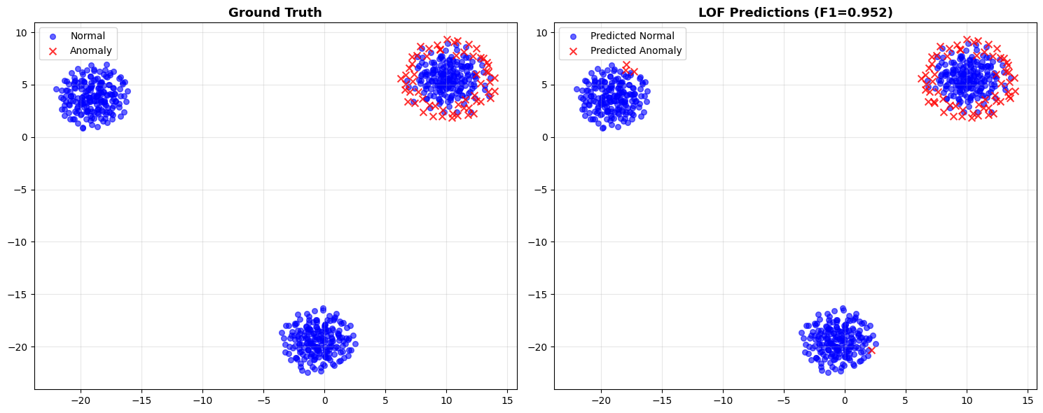
3. Isolation Forest
What is Isolation Forest? An ensemble method that isolates anomalies by building random decision trees. The key insight: anomalies are easier to isolate than normal points, requiring fewer random splits.
The intuition: Imagine randomly drawing lines to separate points. An outlier far from clusters gets isolated quickly (few splits), while a normal point in a dense cluster needs many splits to isolate.
How it works:
Build 100 random trees (n_estimators=100), each selecting random features and split points
For each point, measure its average path length (number of splits to isolate it)
Shorter paths = easier to isolate = likely anomaly
Score is normalized: values close to -1 are anomalies, close to 0 are normal
When to use Isolation Forest:
Large datasets: Scales better than LOF (no pairwise distance computations)
High-dimensional embeddings: Works well with 256-dim TabularResNet embeddings
Fast deployment: No need to tune k parameter (unlike LOF, k-NN)
Baseline comparison: Quick to train, provides reasonable baseline performance
Advantages for OCSF observability data:
✅ Fast training and prediction (tree-based, can parallelize)
✅ Handles curse of dimensionality better than distance-based methods
✅ Detects global outliers effectively (events unlike anything seen before)
✅ No assumptions about data distribution
Disadvantages:
❌ May miss local anomalies (focuses on global outliers)
❌ Sensitive to contamination parameter (must estimate % of anomalies)
❌ Random nature can give inconsistent results (use ensemble averaging)
❌ Less interpretable than distance-based methods
Hyperparameter tuning:
contamination: Set to expected anomaly rate
Too low (0.01) → misses anomalies
Too high (0.2) → many false positives
Start with 0.1 (10% anomalies) and adjust based on domain knowledge
n_estimators: Number of trees
More trees (200) → more stable but slower
Fewer trees (50) → faster but noisier
Default 100 is usually good balance
For observability data: Isolation Forest works well as a first pass to catch obvious outliers before applying more expensive methods like LOF.
from sklearn.ensemble import IsolationForest

def detect_anomalies_iforest(embeddings, contamination=0.1, n_estimators=100):
    """
    Detect anomalies using Isolation Forest.

    Args:
        embeddings: Embedding vectors
        contamination: Expected proportion of anomalies
        n_estimators: Number of trees

    Returns:
        predictions, scores
    """
    iforest = IsolationForest(
        contamination=contamination,
        n_estimators=n_estimators,
        random_state=42,
        n_jobs=-1
    )

    predictions = iforest.fit_predict(embeddings)
    scores = iforest.score_samples(embeddings)  # Lower = more anomalous

    return predictions, scores

# Detect anomalies
predictions_if, scores_if = detect_anomalies_iforest(all_embeddings, contamination=0.1)

# Convert predictions
predicted_labels_if = (predictions_if == -1).astype(int)

# Evaluate
precision_if = precision_score(true_labels, predicted_labels_if)
recall_if = recall_score(true_labels, predicted_labels_if)
f1_if = f1_score(true_labels, predicted_labels_if)

print(f"Isolation Forest Results:")
print(f"  Precision: {precision_if:.3f}")
print(f"  Recall:    {recall_if:.3f}")
print(f"  F1-Score:  {f1_if:.3f}")
Isolation Forest Results:
Precision: 0.909
Recall: 1.000
F1-Score: 0.952
4. Distance-Based Methods
k-NN Distance
What is k-NN distance? A simple but effective method: compute the distance from each point to its k-th nearest neighbor. Points far from their neighbors are anomalies.
The intuition: Normal OCSF events have similar historical events nearby (e.g., previous logins by same user). Anomalies don’t have similar neighbors, so their k-NN distance is large.
How it works:
For each event embedding, find k nearest neighbors in vector DB
Compute distance to the k-th neighbor (not 1st, to avoid noise)
Set a threshold (e.g., 90th percentile of all distances)
Events with distance > threshold are anomalies
Why k-th neighbor, not 1st?
1st neighbor: Too sensitive to noise (one similar point → normal score)
k-th neighbor (k=5-20): More robust, requires multiple similar events to be considered normal
Average of k neighbors: Even more stable but slower to compute
When to use k-NN distance:
Vector DB architecture: You’re already retrieving neighbors, so distance is free
Interpretable results: “This request has no similar requests in the past 30 days” is easy to explain
Real-time detection: Fast lookup in vector DB, immediate scoring
Baseline method: Simple to implement and understand
Advantages for OCSF observability data:
✅ Directly maps to vector DB operations: retrieve k neighbors → compute distance → score
✅ Easy to explain to operations teams: “No similar events found”
✅ Works well with time windows: Only compare to recent events (last 7 days)
✅ Low latency: Single vector DB query per event
Disadvantages:
❌ Sensitive to k choice (too small = noisy, too large = misses anomalies)
❌ Requires threshold tuning (90th, 95th, 99th percentile?)
❌ Assumes similar distances across all event types (may need per-type thresholds)
❌ Outliers can pollute the database (need to filter detected anomalies)
Hyperparameter tuning:
k (number of neighbors):
k=5: Sensitive, good for rare events
k=20: Robust, recommended starting point
k=50: Very conservative, may miss subtle anomalies
threshold_percentile:
90th: 10% flagged as anomalies (high recall, more false positives)
95th: 5% flagged (balanced)
99th: 1% flagged (high precision, may miss anomalies)
Distance metrics (supported by vector DBs):
Cosine similarity: Good for directional differences (e.g., different user behavior patterns)
Euclidean (L2): Good for magnitude differences (e.g., 10x more bytes than normal)
Negative inner product: Fast approximation of cosine for normalized embeddings
Interpretation:
Distance < threshold: Normal event (has similar historical events)
Distance > threshold: Anomaly (no similar events in history)
Distance >> threshold (2-3x): Strong anomaly signal (investigate immediately)
For observability data: k-NN distance is the most common production method because it:
Leverages existing vector DB infrastructure
Provides intuitive explanations for operations teams
Scales to millions of events with approximate nearest neighbor search
from sklearn.neighbors import NearestNeighbors

def detect_anomalies_knn(embeddings, k=5, threshold_percentile=90):
    """
    Detect anomalies using k-NN distance.

    Args:
        embeddings: Embedding vectors
        k: Number of nearest neighbors
        threshold_percentile: Percentile for anomaly threshold

    Returns:
        predictions, scores
    """
    # Fit k-NN
    nbrs = NearestNeighbors(n_neighbors=k+1)  # +1 because point itself is included
    nbrs.fit(embeddings)

    # Compute distances to k-th nearest neighbor
    distances, indices = nbrs.kneighbors(embeddings)
    knn_distances = distances[:, -1]  # Distance to k-th neighbor

    # Threshold: anomalies are in top (100-threshold_percentile)%
    threshold = np.percentile(knn_distances, threshold_percentile)
    predictions = (knn_distances > threshold).astype(int)

    return predictions, knn_distances

# Detect anomalies
predicted_labels_knn, scores_knn = detect_anomalies_knn(all_embeddings, k=5, threshold_percentile=90)

# Evaluate
precision_knn = precision_score(true_labels, predicted_labels_knn)
recall_knn = recall_score(true_labels, predicted_labels_knn)
f1_knn = f1_score(true_labels, predicted_labels_knn)

print(f"k-NN Distance Results:")
print(f"  Precision: {precision_knn:.3f}")
print(f"  Recall:    {recall_knn:.3f}")
print(f"  F1-Score:  {f1_knn:.3f}")
k-NN Distance Results:
Precision: 0.909
Recall: 1.000
F1-Score: 0.952
4. Supported Similarity Metrics
For vector DB–driven retrieval, stick to metrics supported by VAST Vector DB:
Cosine similarity
Euclidean distance (L2)
Negative inner product
Use one of these metrics consistently across indexing, retrieval, and scoring to keep anomaly thresholds stable.
5. Clustering-Based Anomaly Detection
What is clustering-based detection? First cluster your embeddings into groups (e.g., k-means), then flag points far from any cluster centroid as anomalies.
The intuition: Normal OCSF events form natural clusters (login events, file access, network connections, etc.). Anomalies don’t fit into any cluster and appear far from all centroids.
How it works:
Run k-means clustering on historical embeddings (e.g., k=5 clusters)
For each event, compute distance to nearest cluster centroid
Events far from all centroids (> 95th percentile) are anomalies
Can update clusters periodically (weekly) as data distribution shifts
When to use clustering-based detection:
Known event types: Your OCSF data has clear categories (authentication, file ops, network, etc.)
Stable patterns: Event distributions don’t change rapidly (daily clustering is stable)
Explainability: Can label clusters and say “event doesn’t match any known pattern”
Preprocessing for other methods: Cluster first, then apply LOF within clusters
Advantages for OCSF observability data:
✅ Semantic clustering: Clusters often match natural event types (API calls, database queries, background jobs)
✅ Per-cluster thresholds: Can tune detection sensitivity per event type
✅ Drift detection: Cluster shifts over time indicate changing system behavior
✅ Efficient: Single distance computation per event (to nearest centroid)
Disadvantages:
❌ Must choose k (number of clusters) - wrong k → poor performance
❌ Assumes spherical clusters (k-means limitation)
❌ Misses anomalies within clusters (only detects inter-cluster anomalies)
❌ Sensitive to cluster updates (re-clustering can change detection behavior)
Hyperparameter tuning:
n_clusters (k):
Too few (k=3): Clusters are too broad, many anomalies missed
Too many (k=20): Over-segmentation, normal events flagged as anomalies
Recommendation: Use Silhouette Score from Part 5 to choose k
Observability heuristic: k = number of OCSF event types you expect (typically 5-10)
threshold_percentile:
90th: Aggressive detection (10% flagged)
95th: Balanced (5% flagged) - recommended starting point
99th: Conservative (1% flagged)
Cluster interpretation for observability:
Cluster 0: “Normal API requests” (centroid = typical request pattern)
Cluster 1: “Error responses” (centroid = failed operation pattern)
Cluster 2: “Admin operations” (centroid = configuration changes)
Cluster 3: “Bulk data operations” (centroid = large data transfers)
Anomaly: Event far from all cluster centroids → investigate
Combining with other methods:
Hierarchical: First cluster, then apply LOF within each cluster (catches local anomalies)
Cascade: First clustering (fast), then k-NN (expensive) only for events flagged by clustering
Ensemble: Average scores from clustering, LOF, and k-NN for more robust detection
Operational considerations:
Cluster update frequency: Weekly or monthly (too frequent → unstable, too rare → stale)
Incremental clustering: For streaming data, use online k-means to avoid full retraining
Cluster drift monitoring: Track cluster centroids over time - large shifts indicate concept drift
For observability data: Clustering works well as a pre-filter before expensive methods, or when you want explainable clusters that map to known event types.
from sklearn.cluster import KMeans

def detect_anomalies_clustering(embeddings, n_clusters=3, threshold_percentile=95):
    """
    Detect anomalies as points far from cluster centroids.

    Args:
        embeddings: Embedding vectors
        n_clusters: Number of clusters
        threshold_percentile: Distance percentile for anomaly threshold

    Returns:
        predictions, scores
    """
    # Fit k-means
    kmeans = KMeans(n_clusters=n_clusters, random_state=42, n_init=10)
    kmeans.fit(embeddings)

    # Compute distance to nearest cluster centroid
    distances_to_centroids = np.min(kmeans.transform(embeddings), axis=1)

    # Threshold
    threshold = np.percentile(distances_to_centroids, threshold_percentile)
    predictions = (distances_to_centroids > threshold).astype(int)

    return predictions, distances_to_centroids

# Detect anomalies
predicted_labels_cluster, scores_cluster = detect_anomalies_clustering(
    all_embeddings, n_clusters=3, threshold_percentile=95
)

# Evaluate
precision_cluster = precision_score(true_labels, predicted_labels_cluster)
recall_cluster = recall_score(true_labels, predicted_labels_cluster)
f1_cluster = f1_score(true_labels, predicted_labels_cluster)

print(f"Clustering-Based Results:")
print(f"  Precision: {precision_cluster:.3f}")
print(f"  Recall:    {recall_cluster:.3f}")
print(f"  F1-Score:  {f1_cluster:.3f}")
Clustering-Based Results:
Precision: 1.000
Recall: 0.550
F1-Score: 0.710
6. Multi-Record Sequence Anomaly Detection (Optional - Advanced)
Note: This section covers an optional advanced technique that goes beyond the core “vector DB only” architecture described in this series.
When to Use This Approach
The methods above (LOF, Isolation Forest, k-NN, clustering) detect anomalies in individual events using vector DB similarity search. However, some anomalies only appear when looking at sequences of events:
Use cases for sequence-based detection:
Cascading failures: Each step looks normal individually, but the sequence indicates a problem (e.g., deployment → memory spike → GC pressure → connection pool exhaustion)
Performance degradation patterns: Gradual deterioration over time (e.g., slow memory leak, thread pool exhaustion)
Time-ordered patterns: Anomalies that depend on temporal order, not just individual event features
Trade-offs
Advantages:
Captures temporal dependencies that vector DB methods miss
Can detect subtle cascading failures that evade single-event detection
Learns normal sequence patterns from data
Disadvantages:
Requires training a separate ML model (LSTM) - adds complexity beyond the vector DB only approach
Needs labeled sequence data for training (normal vs anomalous sequences)
Higher latency (must buffer events into sequences before scoring)
More infrastructure to maintain (model training, versioning, monitoring)
Recommendation: Start with vector DB methods (Sections 1-5). For cascading failure detection:
Prefer the agentic approach (Part 9: Agentic RCA) - uses semantic search and reasoning to detect multi-step patterns without training an LSTM
Use LSTM (shown below) only when you need sub-second latency or purely statistical pattern detection
Alternative: Agentic Multi-Step Detection
For most teams, the agentic approach in Part 9 is preferable to LSTM for detecting cascading failures:
Why agentic approach is better:
✅ No separate model to train/maintain (uses existing vector DB)
✅ Robust to timing variations (semantic similarity vs. exact temporal patterns)
✅ Explainable reasoning (shows investigation trace)
✅ Works with few examples (one-shot learning via historical search)
✅ Incorporates business logic (can reason about workflows)
When to use LSTM instead:
Need sub-millisecond latency
Purely statistical patterns without semantic meaning
Have large labeled sequence datasets
See Part 9: Agentic Sequence Investigation for the recommended approach.
LSTM Implementation (Optional)
For teams that need ultra-low latency or have specific requirements for neural sequence modeling:
For detecting anomalies across sequences of events (e.g., cascading operational failures).
import torch
import torch.nn as nn

class SequenceAnomalyDetector(nn.Module):
    """
    Detect anomalies in sequences of events using embeddings.
    """
    def __init__(self, embedding_dim, hidden_dim=128):
        super().__init__()

        # LSTM to model sequences of embeddings
        self.lstm = nn.LSTM(embedding_dim, hidden_dim, num_layers=2,
                           batch_first=True, dropout=0.1)

        # Predict "normality score"
        self.scorer = nn.Sequential(
            nn.Linear(hidden_dim, 64),
            nn.ReLU(),
            nn.Linear(64, 1),
            nn.Sigmoid()  # Output probability of being normal
        )

    def forward(self, sequence_embeddings):
        """
        Args:
            sequence_embeddings: (batch_size, sequence_length, embedding_dim)

        Returns:
            normality_scores: (batch_size,) probability of sequence being normal
        """
        # Process sequence
        lstm_out, (hidden, cell) = self.lstm(sequence_embeddings)

        # Use final hidden state for scoring
        score = self.scorer(hidden[-1])

        return score.squeeze()

# Example usage
sequence_detector = SequenceAnomalyDetector(embedding_dim=256, hidden_dim=128)

# Simulate a sequence of 10 events
sequence = torch.randn(1, 10, 256)  # 1 sequence, 10 events, 256-dim embeddings
normality_score = sequence_detector(sequence)

print(f"\nSequence Anomaly Detection:")
print(f"  Sequence shape: {sequence.shape}")
print(f"  Normality score: {normality_score.item():.3f}")
print(f"  Interpretation: Lower score = more likely anomaly sequence")
print(f"\nUse case: Detect cascading failures or performance degradation patterns")
Sequence Anomaly Detection:
  Sequence shape: torch.Size([1, 10, 256])
  Normality score: 0.503
  Interpretation: Lower score = more likely anomaly sequence

Use case: Detect cascading failures or performance degradation patterns
7. Method Comparison
Why compare methods? Each anomaly detection algorithm (LOF, Isolation Forest, k-NN, Clustering) has different strengths and weaknesses. A systematic comparison on your specific OCSF data tells you which method works best for your operational patterns.
What this section does:
Runs all four methods on the same embedding dataset
Computes precision, recall, and F1-score for each
Ranks methods by F1-score (balanced metric)
Helps you choose the best algorithm for your observability data
How to interpret results:
High precision, low recall: Method is conservative (few false alarms, but misses some issues)
Low precision, high recall: Method is aggressive (catches everything, but many false alarms)
High F1-score: Best balance for most teams
Typical results for OCSF observability data:
Isolation Forest: Often ranks #1 for high-dimensional embeddings (256-dim)
LOF: Strong for datasets with varying density patterns (mix of frequent/rare events)
k-NN Distance: Simple and interpretable, good baseline
Clustering: Works well when you have distinct operational modes
Next steps after comparison: Use the winning method’s threshold tuning (Section 8) to optimize for your team’s precision/recall priorities.
def compare_anomaly_methods(embeddings, true_labels):
    """
    Compare all anomaly detection methods.

    Args:
        embeddings: Embedding vectors
        true_labels: Ground truth (0=normal, 1=anomaly)

    Returns:
        Comparison DataFrame
    """
    results = []

    # LOF
    pred_lof, _ = detect_anomalies_lof(embeddings, contamination=0.1)
    pred_lof = (pred_lof == -1).astype(int)
    results.append({
        'Method': 'Local Outlier Factor',
        'Precision': precision_score(true_labels, pred_lof),
        'Recall': recall_score(true_labels, pred_lof),
        'F1-Score': f1_score(true_labels, pred_lof)
    })

    # Isolation Forest
    pred_if, _ = detect_anomalies_iforest(embeddings, contamination=0.1)
    pred_if = (pred_if == -1).astype(int)
    results.append({
        'Method': 'Isolation Forest',
        'Precision': precision_score(true_labels, pred_if),
        'Recall': recall_score(true_labels, pred_if),
        'F1-Score': f1_score(true_labels, pred_if)
    })

    # k-NN Distance
    pred_knn, _ = detect_anomalies_knn(embeddings, k=5)
    results.append({
        'Method': 'k-NN Distance',
        'Precision': precision_score(true_labels, pred_knn),
        'Recall': recall_score(true_labels, pred_knn),
        'F1-Score': f1_score(true_labels, pred_knn)
    })

    # Clustering
    pred_cluster, _ = detect_anomalies_clustering(embeddings, n_clusters=3)
    results.append({
        'Method': 'Clustering-Based',
        'Precision': precision_score(true_labels, pred_cluster),
        'Recall': recall_score(true_labels, pred_cluster),
        'F1-Score': f1_score(true_labels, pred_cluster)
    })

    # Sort by F1-Score
    results = sorted(results, key=lambda x: x['F1-Score'], reverse=True)

    # Print comparison table
    print("\n" + "="*70)
    print("ANOMALY DETECTION METHOD COMPARISON")
    print("="*70)
    print(f"{'Rank':<6} {'Method':<25} {'Precision':<12} {'Recall':<12} {'F1-Score':<12}")
    print("-"*70)
    for i, r in enumerate(results, 1):
        print(f"{i:<6} {r['Method']:<25} {r['Precision']:<12.3f} {r['Recall']:<12.3f} {r['F1-Score']:<12.3f}")
    print("="*70)

    return results

# Run comparison
comparison_results = compare_anomaly_methods(all_embeddings, true_labels)
======================================================================
ANOMALY DETECTION METHOD COMPARISON
======================================================================
Rank   Method                    Precision    Recall       F1-Score
----------------------------------------------------------------------
1      Local Outlier Factor      0.909        1.000        0.952
2      Isolation Forest          0.909        1.000        0.952
3      k-NN Distance             0.909        1.000        0.952
4      Clustering-Based          1.000        0.550        0.710
======================================================================
8. Threshold Tuning
Why threshold tuning matters: All anomaly detection methods require setting a threshold - the cutoff between “normal” and “anomaly”. Too low → miss operational issues (low recall). Too high → false alarms (low precision).
The challenge: Operations teams have different priorities:
Site Reliability Engineers (SREs): Want high precision (few false alarms to investigate)
Platform teams: Want high recall (catch all degradation early)
Production systems: Need balance based on investigation capacity
Precision-Recall trade-off:
High threshold (99th percentile): Only flag clear outliers → High precision, low recall (misses subtle issues)
Low threshold (90th percentile): Flag more events → High recall, low precision (many false positives)
Sweet spot: Find threshold that balances precision/recall for your use case
Example scenarios:
Critical services (payment processing): High recall (95%) > precision. Can’t miss performance degradation.
Log analysis (general monitoring): Balanced (F1 score). Limited investigation capacity.
Alert fatigue prevention: High precision (90%) > recall. Operations team overwhelmed by alerts.
Precision-Recall Curve
What is a PR curve? A plot showing precision vs recall at different thresholds. Use it to visualize the trade-off and select the optimal threshold for your operations team’s priorities.
How to read it:
Top-right corner: Ideal (high precision AND high recall) - rarely achievable
Top-left: High precision, low recall (few alerts, might miss issues)
Bottom-right: Low precision, high recall (many alerts, catch everything)
Area under curve (AUC): Overall method quality (higher = better across all thresholds)
Interpretation:
AUC > 0.9: Excellent - method works well regardless of threshold
AUC 0.7-0.9: Good - can find acceptable threshold
AUC < 0.7: Poor - consider different method or improve embeddings
For observability data: Choose threshold based on your investigation capacity:
Can investigate 10 alerts/day? → Set threshold for 10 flagged events/day
Must catch all degradation? → Set threshold for 95% recall, accept higher false positives
from sklearn.metrics import precision_recall_curve, auc

def plot_precision_recall_curve(true_labels, scores, method_name):
    """
    Plot precision-recall curve for threshold tuning.

    Args:
        true_labels: Ground truth
        scores: Anomaly scores (higher = more anomalous)
        method_name: Name of the method
    """
    precision, recall, thresholds = precision_recall_curve(true_labels, scores)
    pr_auc = auc(recall, precision)

    plt.figure(figsize=(8, 6))
    plt.plot(recall, precision, linewidth=2, label=f'{method_name} (AUC={pr_auc:.3f})')
    plt.xlabel('Recall', fontsize=12)
    plt.ylabel('Precision', fontsize=12)
    plt.title(f'Precision-Recall Curve: {method_name}', fontsize=14, fontweight='bold')
    plt.legend()
    plt.grid(True, alpha=0.3)
    plt.tight_layout()
    plt.show()

    print(f"\nPrecision-Recall AUC: {pr_auc:.3f}")
    print(f"Use this curve to select the best threshold for your use case")

# Example: Plot PR curve for k-NN distance
plot_precision_recall_curve(true_labels, scores_knn, "k-NN Distance")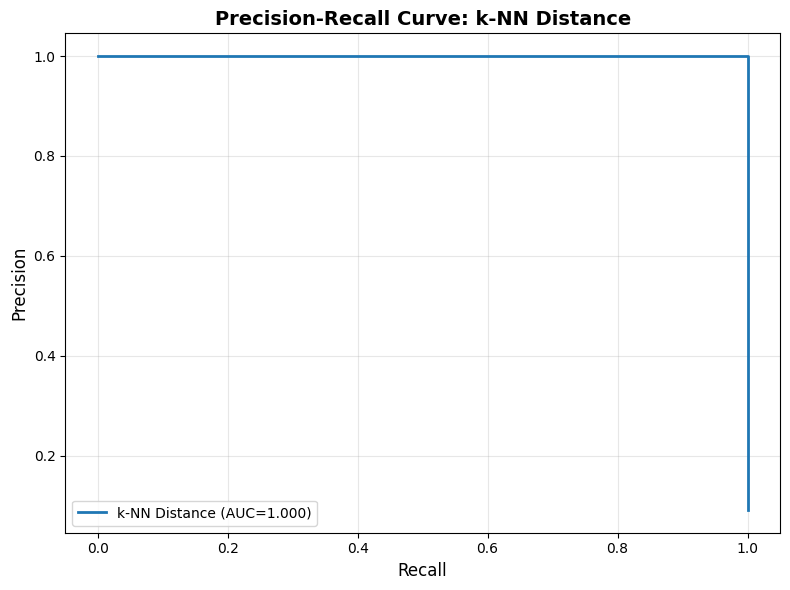
Precision-Recall AUC: 1.000
Use this curve to select the best threshold for your use case
9. Production Pipeline
Why a production pipeline matters: Combining all the pieces (preprocessing, embedding generation, anomaly detection, alerting) into a single, deployable system.
The end-to-end flow:
Ingest: Receive OCSF events from log collectors (Splunk, Kafka, etc.)
Preprocess: Extract features, apply scaler/encoders from Part 3
Embed: Generate 256-dim embedding using trained TabularResNet
Retrieve: Query vector DB for k nearest neighbors
Score: Apply anomaly detection algorithm (LOF, k-NN, etc.)
Alert: If score > threshold, send to SIEM/ticketing system
Store: Persist embedding in vector DB for future comparisons (if not anomaly)
Key design decisions:
Stateful vs Stateless:
Stateful (LOF, Isolation Forest): Pre-fitted on historical data, used for prediction
Stateless (k-NN distance): No pre-fitting, query vector DB directly
Recommendation: Start with stateless k-NN (simpler, scales better)
Online vs Batch:
Online (real-time): Process each event as it arrives (<100ms latency)
Batch (offline): Process events in batches every 5 minutes
Observability context: Most operational issues span minutes/hours, so 5-min batches are acceptable
Novelty detection mode:
Fit once on clean historical data (normal events only)
Predict on new events (don’t retrain on anomalies)
LOF novelty=True enables this mode for streaming data
Error handling:
Missing features → use defaults or skip (don’t crash pipeline)
Model timeout → fall back to rule-based detection
Vector DB down → buffer events, replay when recovered
Operational monitoring:
Throughput: Events/second processed (target: >1000/sec)
Latency: P95 detection latency (target: <500ms)
Alert rate: Anomalies flagged per day (should be stable, spikes indicate issues)
False positive rate: % of alerts dismissed by operations team (track via incident feedback)
For observability data: Production pipeline must be reliable (no events dropped), fast (detect issues within minutes), and explainable (provide context for each alert).
Complete Anomaly Detection Pipeline
What this code provides: A reusable class that wraps TabularResNet + preprocessing + anomaly detection, ready for integration with your observability infrastructure.
class AnomalyDetectionPipeline:
    """
    Production-ready anomaly detection pipeline.
    """
    def __init__(self, model, scaler, encoders, method='lof', contamination=0.1):
        """
        Args:
            model: Trained TabularResNet
            scaler: Fitted StandardScaler for numerical features
            encoders: Dict of LabelEncoders for categorical features
            method: 'lof', 'iforest', 'knn', or 'ensemble'
            contamination: Expected anomaly rate
        """
        self.model = model
        self.scaler = scaler
        self.encoders = encoders
        self.method = method
        self.contamination = contamination
        self.detector = None

    def fit(self, embeddings):
        """Fit the anomaly detector on normal data."""
        if self.method == 'lof':
            self.detector = LocalOutlierFactor(
                n_neighbors=20,
                contamination=self.contamination,
                novelty=True  # For online prediction
            )
        elif self.method == 'iforest':
            self.detector = IsolationForest(
                contamination=self.contamination,
                random_state=42,
                n_jobs=-1
            )
        elif self.method == 'knn':
            self.detector = NearestNeighbors(n_neighbors=5)

        self.detector.fit(embeddings)
        print(f"Anomaly detector ({self.method}) fitted on {len(embeddings)} samples")

    def predict(self, ocsf_records):
        """
        Predict anomalies for new OCSF records.

        Args:
            ocsf_records: List of OCSF dictionaries or DataFrame

        Returns:
            predictions: Binary array (1=anomaly, 0=normal)
            scores: Anomaly scores
        """
        # TODO: Implement preprocessing and embedding extraction
        # This is a simplified example
        pass

print("AnomalyDetectionPipeline class defined")
print("Usage:")
print("  pipeline = AnomalyDetectionPipeline(model, scaler, encoders, method='lof')")
print("  pipeline.fit(training_embeddings)")
print("  predictions, scores = pipeline.predict(new_ocsf_records)")
AnomalyDetectionPipeline class defined
Usage:
pipeline = AnomalyDetectionPipeline(model, scaler, encoders, method='lof')
pipeline.fit(training_embeddings)
predictions, scores = pipeline.predict(new_ocsf_records)
Summary
In this part, you learned:
Core vector DB approach: Five scoring algorithms (LOF, Isolation Forest, k-NN, clustering) that work directly on TabularResNet embeddings—no additional model training required
Method comparison framework for selecting the best approach
Threshold tuning using precision-recall curves
Production pipeline for real-time anomaly detection
Optional advanced extension: LSTM-based sequence anomaly detection for cascading failures (requires training a separate model)
Key Takeaways:
Vector DB only: The core architecture uses TabularResNet embeddings + scoring algorithms—no separate detection model
Isolation Forest works well for high-dimensional embeddings
LOF is good for detecting local density deviations
Ensemble methods combining multiple detectors often perform best
Tune thresholds based on your precision/recall requirements
Sequence detection: Only add if you need multi-event pattern detection (adds model training complexity)
Next: In Part 7, we’ll deploy this system to production with REST APIs for embedding model serving and integration with observability platforms.
Advanced Extension: For production systems with multiple observability data sources (logs, metrics, traces, configuration changes), see Part 9: Multi-Source Correlation to learn how to correlate anomalies across sources and automatically identify root causes.