Theory: See Part 4: Self-Supervised Training for the concepts behind contrastive learning.
Train TabularResNet on OCSF data using self-supervised contrastive learning.
What you’ll learn:
Contrastive learning for tabular data
Data augmentation strategies for OCSF events
Training loop implementation
Extracting embeddings for downstream tasks
Prerequisites:
Processed features from 03
-feature -engineering .ipynb PyTorch installed
Key Concept: Self-Supervised Learning
Problem: We have millions of OCSF logs but no labels (normal vs anomaly).
Solution: Self-supervised learning creates a training signal from the data itself:
Take a log event and create two augmented versions (add noise, mask features)
Train the model to recognize that both versions came from the same event
The model learns meaningful representations without needing labels
import numpy as np
import pickle
import torch
import torch.nn as nn
import torch.nn.functional as F
from torch.utils.data import DataLoader, TensorDataset
import matplotlib.pyplot as plt
import warnings
warnings.filterwarnings('ignore')

# Check for GPU
device = torch.device('cuda' if torch.cuda.is_available() else 'cpu')
print(f"Using device: {device}")
if device.type == 'cuda':
    print(f"  GPU: {torch.cuda.get_device_name(0)}")
else:
    print("  (Training will be slower on CPU, but still works fine for this dataset)")
Using device: cpu
(Training will be slower on CPU, but still works fine for this dataset)
1. Load Processed Features
Load the numerical and categorical feature arrays from the feature engineering notebook.
What you should expect:
Numerical features:
(N, 9)- normalized floatsCategorical features:
(N, 12)- integer indicesCardinalities: list of vocab sizes for each categorical column
If you see errors:
FileNotFoundError: Run notebook 03 first to generate the feature filesShape mismatch: Ensure you’re using the same data version
# Load feature arrays
numerical = np.load('../data/numerical_features.npy')
categorical = np.load('../data/categorical_features.npy')

# Load artifacts (encoders, scaler, cardinalities)
with open('../data/feature_artifacts.pkl', 'rb') as f:
    artifacts = pickle.load(f)

cardinalities = artifacts['cardinalities']

print("Loaded Features:")
print(f"  Numerical: {numerical.shape} (float32)")
print(f"  Categorical: {categorical.shape} (int64)")
print(f"  Cardinalities: {cardinalities}")
print(f"  Total embedding params: {sum(c * 32 for c in cardinalities):,}")
Loaded Features:
Numerical: (27084, 9) (float32)
Categorical: (27084, 12) (int64)
Cardinalities: [2, 4, 3, 3, 2, 7, 4, 2281, 4, 4, 3, 3]
Total embedding params: 74,240
# Convert to PyTorch tensors
numerical_tensor = torch.tensor(numerical, dtype=torch.float32)
categorical_tensor = torch.tensor(categorical, dtype=torch.long)

# Create dataset and dataloader
# Large batches are IMPORTANT for contrastive learning (more negatives)
dataset = TensorDataset(numerical_tensor, categorical_tensor)
batch_size = 256
dataloader = DataLoader(dataset, batch_size=batch_size, shuffle=True, drop_last=True)

print(f"\nDataLoader:")
print(f"  Dataset size: {len(dataset):,} events")
print(f"  Batch size: {batch_size}")
print(f"  Batches per epoch: {len(dataloader)}")
print(f"  (drop_last=True: last incomplete batch dropped)")
DataLoader:
  Dataset size: 27,084 events
  Batch size: 256
  Batches per epoch: 105
  (drop_last=True: last incomplete batch dropped)
2. Define TabularResNet Model
A ResNet-style architecture adapted for tabular data:
Categorical embeddings: Convert integer indices to dense vectors
Input projection: Combine numerical + embedded categorical features
Residual blocks: Deep feature learning with skip connections
Output: 192-dimensional embedding vector
What you should expect:
~100K-500K parameters (depends on cardinalities)
Model fits easily in memory (even on CPU)
If model is too large:
Reduce
embedding_dim(32 -> 16)Reduce
d_model(192 -> 128)Reduce
num_blocks(6 -> 4)
class ResidualBlock(nn.Module):
    """Residual block with two linear layers and skip connection."""

    def __init__(self, d_model, dropout=0.15):
        super().__init__()
        self.linear1 = nn.Linear(d_model, d_model)
        self.linear2 = nn.Linear(d_model, d_model)
        self.norm1 = nn.LayerNorm(d_model)
        self.norm2 = nn.LayerNorm(d_model)
        self.dropout = nn.Dropout(dropout)

    def forward(self, x):
        # Pre-norm residual connection
        residual = x
        x = self.norm1(x)
        x = F.gelu(self.linear1(x))
        x = self.dropout(x)
        x = self.norm2(x)
        x = self.linear2(x)
        x = self.dropout(x)
        return x + residual  # Skip connection


class TabularResNet(nn.Module):
    """
    ResNet-style architecture for tabular data.

    Architecture:
        Input -> [Cat Embeddings + Numerical] -> Projection -> ResBlocks -> Output
    """

    def __init__(self, num_numerical, cardinalities, d_model=192,
                 num_blocks=6, embedding_dim=32, dropout=0.15):
        super().__init__()

        self.d_model = d_model

        # Categorical embeddings: one embedding layer per categorical feature
        self.embeddings = nn.ModuleList([
            nn.Embedding(cardinality, embedding_dim)
            for cardinality in cardinalities
        ])

        # Calculate input dimension
        total_cat_dim = len(cardinalities) * embedding_dim
        input_dim = num_numerical + total_cat_dim

        # Input projection to model dimension
        self.input_projection = nn.Linear(input_dim, d_model)

        # Stack of residual blocks
        self.blocks = nn.ModuleList([
            ResidualBlock(d_model, dropout)
            for _ in range(num_blocks)
        ])

        # Final layer norm
        self.final_norm = nn.LayerNorm(d_model)

    def forward(self, numerical, categorical, return_embedding=True):
        # Embed each categorical feature
        cat_embedded = []
        for i, emb_layer in enumerate(self.embeddings):
            cat_embedded.append(emb_layer(categorical[:, i]))

        # Concatenate: [numerical, cat_emb_1, cat_emb_2, ...]
        if cat_embedded:
            cat_concat = torch.cat(cat_embedded, dim=1)
            x = torch.cat([numerical, cat_concat], dim=1)
        else:
            x = numerical

        # Project to model dimension
        x = self.input_projection(x)

        # Apply residual blocks
        for block in self.blocks:
            x = block(x)

        # Final normalization
        x = self.final_norm(x)

        return x
# Create model
model = TabularResNet(
num_numerical=numerical.shape[1],
cardinalities=cardinalities,
d_model=128,
num_blocks=4,
embedding_dim=32,
dropout=0.1
).to(device)
# Count parameters
total_params = sum(p.numel() for p in model.parameters())
trainable_params = sum(p.numel() for p in model.parameters() if p.requires_grad)
print("Model Architecture:")
print(f" Input: {numerical.shape[1]} numerical + {len(cardinalities)} categorical features")
print(f" Embedding dim: 32 per categorical")
print(f" Model dim (d_model): 128")
print(f" Residual blocks: 4")
print(f" Output: 128-dimensional embedding")
print(f"\nParameters: {total_params:,} ({trainable_params:,} trainable)")Model Architecture:
Input: 9 numerical + 12 categorical features
Embedding dim: 32 per categorical
Model dim (d_model): 128
Residual blocks: 4
Output: 128-dimensional embedding
Parameters: 259,072 (259,072 trainable)
3. Define Contrastive Learning Components
Contrastive learning (SimCLR-style) trains the model so that:
Positive pairs (augmented versions of same event) → similar embeddings
Negative pairs (different events) → dissimilar embeddings
Data Augmentation for OCSF
We augment tabular data by:
Numerical: Add small Gaussian noise (~15%)
Categorical: Random dropout (~20%) - replace with random value
What we DON’T augment: Operationally-critical fields like status, severity_id, activity_id ideally shouldn’t be heavily augmented (we use light augmentation here for simplicity).
class TabularAugmentation:
    """
    Data augmentation for tabular data.

    For OCSF data:
    - Numerical: Add small Gaussian noise
    - Categorical: Random dropout (replace with random value)
    """

    def __init__(self, noise_level=0.15, dropout_prob=0.20):
        self.noise_level = noise_level
        self.dropout_prob = dropout_prob

    def augment_numerical(self, numerical):
        """Add Gaussian noise to numerical features."""
        noise = torch.randn_like(numerical) * self.noise_level
        return numerical + noise

    def augment_categorical(self, categorical, cardinalities):
        """Randomly replace some categorical features with random values."""
        augmented = categorical.clone()
        mask = torch.rand_like(categorical.float()) < self.dropout_prob

        for i, cardinality in enumerate(cardinalities):
            random_cats = torch.randint(
                0, cardinality, (categorical.size(0),),
                device=categorical.device
            )
            augmented[:, i] = torch.where(
                mask[:, i], random_cats, categorical[:, i]
            )

        return augmented
# Visualize augmentation
augmenter = TabularAugmentation(noise_level=0.15, dropout_prob=0.20)
# Get a sample batch
sample_num, sample_cat = next(iter(dataloader))
# Augment
aug_num = augmenter.augment_numerical(sample_num)
aug_cat = augmenter.augment_categorical(sample_cat, cardinalities)
# Show difference
fig, axes = plt.subplots(1, 2, figsize=(14, 4))
# Numerical: show noise distribution
noise = (aug_num - sample_num).numpy().flatten()
axes[0].hist(noise, bins=50, edgecolor='black', alpha=0.7)
axes[0].axvline(0, color='red', linestyle='--', linewidth=2)
axes[0].set_xlabel('Noise Added')
axes[0].set_ylabel('Count')
axes[0].set_title(f'Numerical Augmentation (noise_level={augmenter.noise_level})')
axes[0].annotate(f'std={noise.std():.3f}', xy=(0.7, 0.9), xycoords='axes fraction')
# Categorical: show dropout rate
changed = (aug_cat != sample_cat).float().mean(dim=0).numpy()
axes[1].bar(range(len(changed)), changed, edgecolor='black')
axes[1].axhline(augmenter.dropout_prob, color='red', linestyle='--',
label=f'target={augmenter.dropout_prob}')
axes[1].set_xlabel('Categorical Feature Index')
axes[1].set_ylabel('Fraction Changed')
axes[1].set_title(f'Categorical Augmentation (dropout={augmenter.dropout_prob})')
axes[1].legend()
plt.tight_layout()
plt.show()
print(f"Numerical: mean noise = {noise.mean():.4f}, std = {noise.std():.4f}")
print(f"Categorical: average {changed.mean()*100:.1f}% of values changed per feature")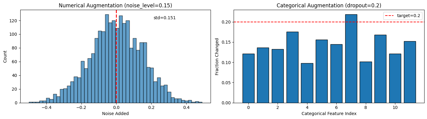
Numerical: mean noise = -0.0018, std = 0.1513
Categorical: average 14.4% of values changed per feature
How to read these augmentation charts
Left (Numerical noise): Histogram of noise values added to numerical features.
Centered at 0 (no bias)
Width controlled by
noise_levelparameterToo wide → augmented views too different → model can’t learn
Too narrow → views too similar → model doesn’t generalize
Right (Categorical dropout): Bar chart showing fraction of values changed per feature.
Red line = target dropout probability (15%)
Bars should hover around the red line
Higher bars = more aggressive augmentation for that feature
def contrastive_loss(model, numerical, categorical, cardinalities,
                     temperature=0.05, augmenter=None):
    """
    SimCLR-style contrastive loss for tabular data.

    For each record in the batch:
    1. Create two augmented views
    2. Compute embeddings for both views
    3. Pull embeddings of same record together (positive pairs)
    4. Push embeddings of different records apart (negative pairs)

    Args:
        temperature: Controls sharpness of similarity distribution
                    Lower = sharper peaks (0.07 is typical)
    """
    if augmenter is None:
        augmenter = TabularAugmentation()

    batch_size = numerical.size(0)

    # Create two augmented views of each record
    num_aug1 = augmenter.augment_numerical(numerical)
    cat_aug1 = augmenter.augment_categorical(categorical, cardinalities)
    emb1 = model(num_aug1, cat_aug1)

    num_aug2 = augmenter.augment_numerical(numerical)
    cat_aug2 = augmenter.augment_categorical(categorical, cardinalities)
    emb2 = model(num_aug2, cat_aug2)

    # Concatenate embeddings: [view1_batch, view2_batch]
    embeddings = torch.cat([emb1, emb2], dim=0)  # (2*batch_size, d_model)

    # L2 normalize (important for cosine similarity)
    embeddings = F.normalize(embeddings, dim=1)

    # Compute similarity matrix
    similarity = torch.matmul(embeddings, embeddings.T) / temperature

    # Labels: positive pairs are (i, i+batch_size) and (i+batch_size, i)
    labels = torch.cat([
        torch.arange(batch_size, 2 * batch_size),
        torch.arange(0, batch_size)
    ], dim=0).to(numerical.device)

    # Mask self-similarity (diagonal)
    mask = torch.eye(2 * batch_size, dtype=torch.bool, device=numerical.device)
    similarity = similarity.masked_fill(mask, float('-inf'))

    # Cross-entropy loss (treat as classification: which is the positive?)
    loss = F.cross_entropy(similarity, labels)

    return loss
# Test the loss function
augmenter = TabularAugmentation(noise_level=0.15, dropout_prob=0.20)
# Get a batch
num_batch, cat_batch = next(iter(dataloader))
num_batch = num_batch.to(device)
cat_batch = cat_batch.to(device)
# Compute loss
with torch.no_grad():
initial_loss = contrastive_loss(model, num_batch, cat_batch, cardinalities, augmenter=augmenter)
print(f"Initial contrastive loss: {initial_loss.item():.4f}")
print(f"\nExpected initial loss: ~{np.log(2 * batch_size - 1):.2f}")
print(f" (Random embeddings should give loss ≈ log(num_negatives))")
print(f"\nGood training should reduce this significantly (target: < 3.0)")Initial contrastive loss: 6.2040
Expected initial loss: ~6.24
(Random embeddings should give loss ≈ log(num_negatives))
Good training should reduce this significantly (target: < 3.0)
4. Training Loop
Train the model using contrastive learning.
What you should expect:
Initial loss: ~5.5 (for batch_size=256, this is log(511) ≈ 6.2)
Loss should decrease steadily each epoch
Final loss: typically 2.0-4.0 (lower = better alignment)
Training time: ~5-8 minutes on CPU, ~1 minute on GPU
If loss doesn’t decrease:
Learning rate too high: try 1e-4 instead of 1e-3
Data issue: verify features are normalized properly
Augmentation too strong: reduce noise_level and dropout_prob
If loss goes to NaN:
Learning rate too high
Numerical instability: check for NaN in features
def train_epoch(model, dataloader, optimizer, cardinalities, augmenter, device):
    """Train for one epoch."""
    model.train()
    total_loss = 0

    for numerical, categorical in dataloader:
        numerical = numerical.to(device)
        categorical = categorical.to(device)

        optimizer.zero_grad()
        loss = contrastive_loss(
            model, numerical, categorical, cardinalities,
            augmenter=augmenter
        )
        loss.backward()
        optimizer.step()

        total_loss += loss.item()

    return total_loss / len(dataloader)
# Training configuration
num_epochs = 80
learning_rate = 1e-3
optimizer = torch.optim.AdamW(model.parameters(), lr=learning_rate, weight_decay=0.01)
scheduler = torch.optim.lr_scheduler.CosineAnnealingLR(optimizer, T_max=num_epochs)
augmenter = TabularAugmentation(noise_level=0.15, dropout_prob=0.20)
print("Training Configuration:")
print(f" Epochs: {num_epochs}")
print(f" Batch size: {batch_size}")
print(f" Learning rate: {learning_rate} (with cosine annealing)")
print(f" Optimizer: AdamW (weight_decay=0.01)")
print(f" Augmentation: noise={augmenter.noise_level}, dropout={augmenter.dropout_prob}")
print("-" * 50)Training Configuration:
Epochs: 80
Batch size: 256
Learning rate: 0.001 (with cosine annealing)
Optimizer: AdamW (weight_decay=0.01)
Augmentation: noise=0.15, dropout=0.2
--------------------------------------------------
# Training loop
losses = []

print("\nStarting training...")
print(f"{'Epoch':>6} | {'Loss':>8} | {'LR':>10} | {'Status'}")
print("-" * 50)

for epoch in range(num_epochs):
    loss = train_epoch(model, dataloader, optimizer, cardinalities, augmenter, device)
    scheduler.step()
    losses.append(loss)

    lr = scheduler.get_last_lr()[0]

    # Determine status
    if epoch == 0:
        status = "Starting"
    elif loss < losses[-2]:
        status = "Improving"
    else:
        status = "Plateau"

    if (epoch + 1) % 5 == 0 or epoch == 0:
        print(f"{epoch+1:>6} | {loss:>8.4f} | {lr:>10.6f} | {status}")

print("-" * 50)
print(f"Final loss: {losses[-1]:.4f}")
print(f"Best loss: {min(losses):.4f} (epoch {losses.index(min(losses))+1})")
Starting training...
 Epoch |     Loss |         LR | Status
--------------------------------------------------
1 | 3.9070 | 0.001000 | Starting
5 | 3.2217 | 0.000990 | Improving
10 | 3.1466 | 0.000962 | Improving
15 | 3.1172 | 0.000916 | Plateau
20 | 3.1049 | 0.000854 | Plateau
25 | 3.0880 | 0.000778 | Plateau
30 | 3.0682 | 0.000691 | Improving
35 | 3.0379 | 0.000598 | Improving
40 | 3.0599 | 0.000500 | Improving
45 | 3.0469 | 0.000402 | Plateau
50 | 3.0405 | 0.000309 | Improving
55 | 3.0574 | 0.000222 | Plateau
60 | 3.0347 | 0.000146 | Plateau
65 | 3.0212 | 0.000084 | Improving
70 | 3.0296 | 0.000038 | Plateau
75 | 3.0157 | 0.000010 | Improving
    80 |   3.0449 |   0.000000 | Plateau
--------------------------------------------------
Final loss: 3.0449
Best loss: 3.0157 (epoch 75)
# Plot training loss
fig, axes = plt.subplots(1, 2, figsize=(14, 5))

# Loss over epochs
axes[0].plot(range(1, len(losses)+1), losses, 'b-', marker='o', markersize=4, linewidth=2)
axes[0].set_xlabel('Epoch')
axes[0].set_ylabel('Contrastive Loss')
axes[0].set_title('Training Loss Over Time')
axes[0].grid(True, alpha=0.3)

# Add reference lines
initial_expected = np.log(2 * batch_size - 1)
axes[0].axhline(initial_expected, color='gray', linestyle='--', alpha=0.5,
               label=f'Random baseline: {initial_expected:.2f}')
axes[0].axhline(3.0, color='green', linestyle='--', alpha=0.5,
               label='Good target: 3.0')
axes[0].legend()

# Loss improvement
improvement = [(losses[0] - l) / losses[0] * 100 for l in losses]
axes[1].bar(range(1, len(losses)+1), improvement, color='steelblue', edgecolor='black')
axes[1].set_xlabel('Epoch')
axes[1].set_ylabel('Improvement from Initial (%)')
axes[1].set_title('Cumulative Training Progress')
axes[1].grid(True, alpha=0.3, axis='y')

plt.tight_layout()
plt.show()

print(f"\nTraining Summary:")
print(f"  Initial loss: {losses[0]:.4f}")
print(f"  Final loss: {losses[-1]:.4f}")
print(f"  Improvement: {(1 - losses[-1]/losses[0])*100:.1f}%")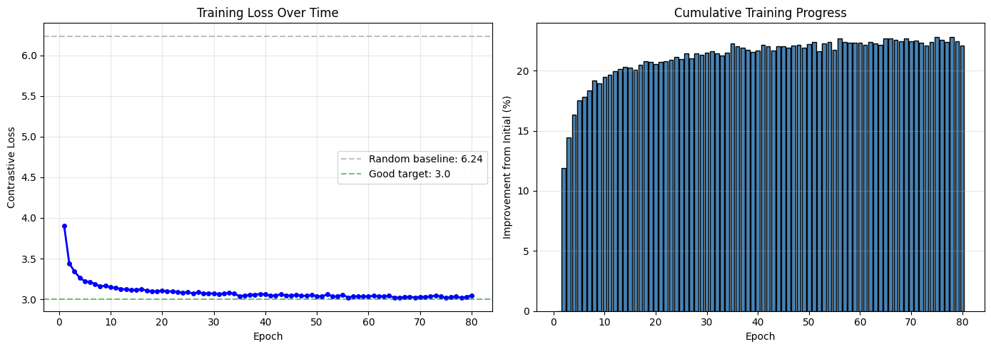
Training Summary:
  Initial loss: 3.9070
  Final loss: 3.0449
  Improvement: 22.1%
How to read the training curves
Left (Loss over time):
Gray dashed line (random baseline): Expected loss if embeddings were random. Loss should start near here.
Green dashed line (target): Good contrastive models reach loss ~3.0 or below.
Blue curve: Should decrease steadily. Plateaus are normal toward the end.
If loss doesn’t decrease: Learning rate may be too high/low, or augmentation too aggressive.
Right (Improvement %):
Shows cumulative improvement from initial loss
Expect 30-50% improvement for well-trained models
Diminishing returns after ~10 epochs is normal
5. Extract Embeddings
Use the trained model to create embeddings for all records.
What you should expect:
Embeddings shape:
(N, 192)- one 192-dim vector per eventValues roughly centered around 0
Similar events should have similar embeddings (high cosine similarity)
@torch.no_grad()
def extract_embeddings(model, numerical, categorical, batch_size=512):
    """
    Extract embeddings for all records.

    Returns:
        numpy array of embeddings (N, d_model)
    """
    model.eval()
    embeddings = []

    dataset = TensorDataset(
        torch.tensor(numerical, dtype=torch.float32),
        torch.tensor(categorical, dtype=torch.long)
    )
    loader = DataLoader(dataset, batch_size=batch_size, shuffle=False)

    for num_batch, cat_batch in loader:
        num_batch = num_batch.to(device)
        cat_batch = cat_batch.to(device)

        emb = model(num_batch, cat_batch)
        embeddings.append(emb.cpu().numpy())

    return np.vstack(embeddings)

# Extract embeddings
print("Extracting embeddings...")
embeddings = extract_embeddings(model, numerical, categorical)

print(f"\nEmbedding Statistics:")
print(f"  Shape: {embeddings.shape}")
print(f"  Mean: {embeddings.mean():.4f}")
print(f"  Std: {embeddings.std():.4f}")
print(f"  Min: {embeddings.min():.4f}")
print(f"  Max: {embeddings.max():.4f}")
Extracting embeddings...
Embedding Statistics:
  Shape: (27084, 128)
  Mean: 0.0025
  Std: 0.9895
  Min: -4.2242
  Max: 4.9933
# Visualize embedding distribution
fig, axes = plt.subplots(1, 3, figsize=(15, 4))

# Distribution of all values
axes[0].hist(embeddings.flatten(), bins=100, edgecolor='black', alpha=0.7)
axes[0].axvline(0, color='red', linestyle='--', linewidth=2)
axes[0].set_xlabel('Embedding Value')
axes[0].set_ylabel('Count')
axes[0].set_title('Distribution of All Embedding Values')

# Distribution of embedding norms
norms = np.linalg.norm(embeddings, axis=1)
axes[1].hist(norms, bins=50, edgecolor='black', alpha=0.7, color='green')
axes[1].set_xlabel('Embedding Norm (L2)')
axes[1].set_ylabel('Count')
axes[1].set_title('Distribution of Embedding Norms')
axes[1].annotate(f'Mean: {norms.mean():.2f}\nStd: {norms.std():.2f}',
                xy=(0.7, 0.8), xycoords='axes fraction')

# Sample embedding dimensions
for i in range(5):
    axes[2].hist(embeddings[:, i], bins=50, alpha=0.5, label=f'dim {i}')
axes[2].set_xlabel('Value')
axes[2].set_ylabel('Count')
axes[2].set_title('Sample Dimension Distributions')
axes[2].legend()

plt.tight_layout()
plt.show()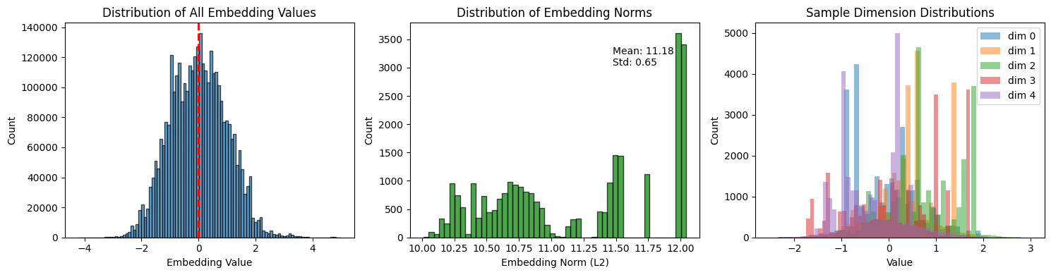
How to read the embedding distributions
Left (All embedding values):
Should be roughly centered around 0 (red dashed line)
Approximately symmetric distribution is healthy
Very long tails may indicate outlier events
Center (Embedding norms):
L2 norm = “length” of the embedding vector
Tight distribution = consistent embedding magnitudes (good)
Wide spread or outliers = some events produce unusual embeddings (potential anomalies)
Right (Individual dimensions):
Shows 5 sample dimensions overlaid
Different dimensions capture different patterns
Highly similar distributions = dimensions may be redundant
# Save embeddings and model
np.save('../data/embeddings.npy', embeddings)
torch.save(model.state_dict(), '../data/tabular_resnet.pt')

print("Saved:")
print(f"  - ../data/embeddings.npy: {embeddings.shape}")
print(f"  - ../data/tabular_resnet.pt: model weights")
Saved:
- ../data/embeddings.npy: (27084, 128)
- ../data/tabular_resnet.pt: model weights
6. Quick Embedding Visualization
Use t-SNE to visualize the learned embedding space in 2D.
What you should expect:
Clusters should form (similar events group together)
Spread indicates diversity in the data
Isolated points may be anomalies
If you see a single blob:
Model may need more training
Try different perplexity values (15, 30, 50)
Data may be very homogeneous
from sklearn.manifold import TSNE

# Sample for visualization (t-SNE is slow on large datasets)
sample_size = min(2000, len(embeddings))
indices = np.random.choice(len(embeddings), sample_size, replace=False)
emb_sample = embeddings[indices]

# Run t-SNE
print(f"Running t-SNE on {sample_size} samples (this may take 1-2 minutes)...")
tsne = TSNE(n_components=2, perplexity=30, random_state=42)
emb_2d = tsne.fit_transform(emb_sample)
print("Done!")
Running t-SNE on 2000 samples (this may take 1-2 minutes)...
Done!
# Plot t-SNE
fig, axes = plt.subplots(1, 2, figsize=(14, 6))

# Basic scatter
axes[0].scatter(emb_2d[:, 0], emb_2d[:, 1], alpha=0.5, s=10, c='steelblue')
axes[0].set_xlabel('t-SNE 1')
axes[0].set_ylabel('t-SNE 2')
axes[0].set_title('OCSF Event Embeddings (t-SNE)')

# Colored by embedding norm (potential anomaly indicator)
norms_sample = np.linalg.norm(emb_sample, axis=1)
scatter = axes[1].scatter(emb_2d[:, 0], emb_2d[:, 1], c=norms_sample,
                          cmap='viridis', alpha=0.5, s=10)
axes[1].set_xlabel('t-SNE 1')
axes[1].set_ylabel('t-SNE 2')
axes[1].set_title('Embeddings Colored by L2 Norm')
plt.colorbar(scatter, ax=axes[1], label='Embedding Norm')

plt.tight_layout()
plt.show()

print("\nInterpretation:")
print("- Clusters = similar events (same activity type, status, etc.)")
print("- Isolated points = potentially unusual events")
print("- High norm (yellow) = events far from center (potential anomalies)")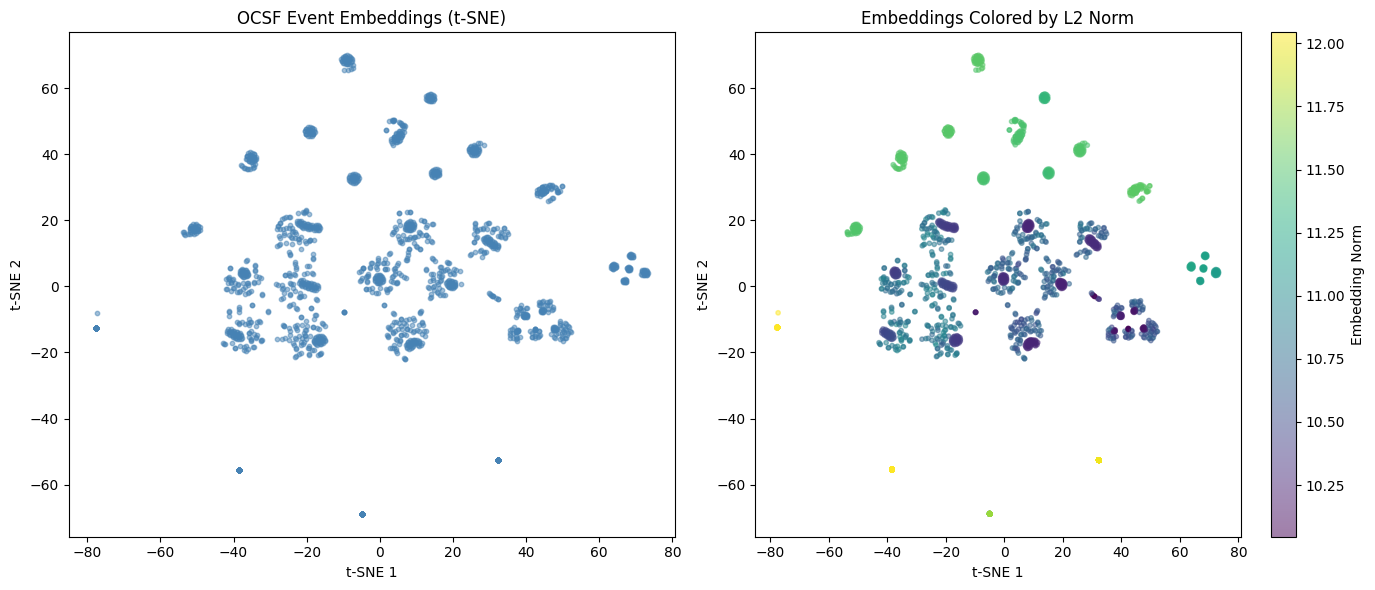
Interpretation:
- Clusters = similar events (same activity type, status, etc.)
- Isolated points = potentially unusual events
- High norm (yellow) = events far from center (potential anomalies)
Summary
In this notebook, we:
Loaded processed features from the feature engineering notebook
Built TabularResNet - categorical embeddings + residual blocks
Implemented contrastive learning - SimCLR-style with tabular augmentation
Trained the model on unlabeled OCSF data (self-supervised)
Extracted embeddings for all records
Visualized the embedding space with t-SNE
Key insight: We learned meaningful representations from unlabeled data by training the model to recognize that augmented versions of the same event should have similar embeddings.
Output files:
embeddings.npy: (N, 192) embedding vectorstabular_resnet.pt: trained model weights
Next:
05
-model -inference .ipynb - Load and use the model for new data 06
-anomaly -detection .ipynb - Detect anomalies using embeddings