Theory: See Part 5: Evaluating Embedding Quality for concepts behind embedding evaluation.
Evaluate the quality of your trained embeddings using both quantitative metrics and qualitative inspection.
What you’ll learn:
Visualize embeddings with t-SNE and UMAP
Inspect nearest neighbors to verify semantic similarity
Compute cluster quality metrics (Silhouette, Davies-Bouldin, Calinski-Harabasz)
Determine optimal number of clusters (k)
Test embedding robustness with perturbation stability
Evaluate k-NN classification as a proxy task
Generate a comprehensive quality report
Prerequisites:
Embeddings from 04
-self -supervised -training .ipynb Trained model (
tabular_resnet.pt)
Why Evaluate Embeddings?
The challenge: Just because your training loss decreased doesn’t mean your embeddings are useful. A model can memorize training data while learning poor representations.
The solution: Evaluate from multiple angles:
Quantitative (objective metrics like Silhouette Score)
Qualitative (visual inspection, nearest neighbors)
Numbers don’t tell the whole story - you need to look at your data!
import numpy as np
import pandas as pd
import pickle
import matplotlib.pyplot as plt
import warnings
warnings.filterwarnings('ignore')

from sklearn.manifold import TSNE
from sklearn.cluster import KMeans
from sklearn.metrics import silhouette_score, davies_bouldin_score, calinski_harabasz_score, silhouette_samples
from sklearn.neighbors import KNeighborsClassifier, NearestNeighbors
from sklearn.model_selection import cross_val_score
from sklearn.preprocessing import StandardScaler

# Optional: UMAP for alternative visualization
try:
    import umap
    UMAP_AVAILABLE = True
except ImportError:
    UMAP_AVAILABLE = False

print("✓ All imports successful")
print("\nLibraries loaded:")
print("  - NumPy for numerical operations")
print("  - Pandas for data manipulation")
print("  - Matplotlib for visualization")
print("  - Scikit-learn for clustering and metrics")
print(f"  - UMAP: {'Available' if UMAP_AVAILABLE else 'Not installed (pip install umap-learn)'}")
✓ All imports successful
Libraries loaded:
- NumPy for numerical operations
- Pandas for data manipulation
- Matplotlib for visualization
- Scikit-learn for clustering and metrics
- UMAP: Available
1. Load Embeddings
Load the embeddings generated in the self-supervised training notebook.
What you should expect:
Shape:
(N, 192)- one 192-dimensional vector per OCSF eventValues roughly centered around 0
No NaN or Inf values
If you see errors:
FileNotFoundError: Run notebook 04 first to generate embeddingsWrong shape: Ensure you’re using the correct embedding file
# Load embeddings
embeddings = np.load('../data/embeddings.npy')

# Load original features (for perturbation testing later)
numerical = np.load('../data/numerical_features.npy')
categorical = np.load('../data/categorical_features.npy')

with open('../data/feature_artifacts.pkl', 'rb') as f:
    artifacts = pickle.load(f)

# Load original OCSF data for inspection
ocsf_df = pd.read_parquet('../data/ocsf_logs.parquet')

# Ensure OCSF data matches embeddings length
if len(ocsf_df) != len(embeddings):
    print(f"⚠ Warning: OCSF data has {len(ocsf_df)} rows but embeddings have {len(embeddings)}")
    print(f"  Truncating to match...")
    ocsf_df = ocsf_df.iloc[:len(embeddings)]

print("Loaded Embeddings:")
print(f"  Shape: {embeddings.shape}")
print(f"  Mean: {embeddings.mean():.4f}")
print(f"  Std: {embeddings.std():.4f}")
print(f"  Range: [{embeddings.min():.4f}, {embeddings.max():.4f}]")
print(f"\n✓ No NaN values: {not np.isnan(embeddings).any()}")
print(f"✓ No Inf values: {not np.isinf(embeddings).any()}")

print(f"\nLoaded OCSF Data:")
print(f"  Events: {len(ocsf_df):,}")
print(f"  Columns: {len(ocsf_df.columns)}")
Loaded Embeddings:
Shape: (27084, 128)
Mean: 0.0003
Std: 0.9949
Range: [-4.1475, 4.4995]
✓ No NaN values: True
✓ No Inf values: True
Loaded OCSF Data:
Events: 27,084
Columns: 59
2. Qualitative Evaluation: t-SNE Visualization
What is t-SNE? A dimensionality reduction technique that projects high-dimensional embeddings (192-dim) to 2D while preserving local structure.
What to look for:
✅ Good: Clear, distinct clusters for different event types
✅ Good: Anomalies appear as scattered outliers
❌ Bad: All points in one giant blob (no structure learned)
❌ Bad: Random scatter with no clusters
Note on coloring: Since our embeddings come from self-supervised learning (unsupervised), we don’t have ground truth class labels. The left plot shows raw structure; the right plot uses embedding norm as an anomaly indicator. Compare with Part 5’s labeled synthetic examples for educational context.
Perplexity parameter: Controls balance between local and global structure
Low (5-15): Focus on local neighborhoods
Medium (30): Default, balanced view
High (50): Emphasize global structure
# Sample for visualization (t-SNE is slow on large datasets)
sample_size = min(3000, len(embeddings))
np.random.seed(42)
indices = np.random.choice(len(embeddings), sample_size, replace=False)
emb_sample = embeddings[indices]

print(f"Sampling {sample_size:,} embeddings for t-SNE visualization")
print(f"(Running t-SNE on full dataset would be too slow)")
print(f"\nRunning t-SNE with perplexity=30... (this may take 1-2 minutes)")
Sampling 3,000 embeddings for t-SNE visualization
(Running t-SNE on full dataset would be too slow)
Running t-SNE with perplexity=30... (this may take 1-2 minutes)
# Run t-SNE
tsne = TSNE(n_components=2, perplexity=30, random_state=42, max_iter=1000)
emb_2d = tsne.fit_transform(emb_sample)
print("✓ t-SNE complete!")
✓ t-SNE complete!
# Visualize t-SNE
fig, axes = plt.subplots(1, 2, figsize=(15, 6))

# Basic scatter
axes[0].scatter(emb_2d[:, 0], emb_2d[:, 1], alpha=0.6, s=20, c='steelblue', edgecolors='none')
axes[0].set_xlabel('t-SNE Dimension 1', fontsize=12)
axes[0].set_ylabel('t-SNE Dimension 2', fontsize=12)
axes[0].set_title('OCSF Event Embeddings (t-SNE)', fontsize=14, fontweight='bold')
axes[0].grid(True, alpha=0.3)

# Colored by embedding norm (potential anomaly indicator)
norms = np.linalg.norm(emb_sample, axis=1)
scatter = axes[1].scatter(emb_2d[:, 0], emb_2d[:, 1], c=norms,
                          cmap='viridis', alpha=0.6, s=20, edgecolors='none')
axes[1].set_xlabel('t-SNE Dimension 1', fontsize=12)
axes[1].set_ylabel('t-SNE Dimension 2', fontsize=12)
axes[1].set_title('Colored by Embedding Norm (Anomaly Indicator)', fontsize=14, fontweight='bold')
axes[1].grid(True, alpha=0.3)
cbar = plt.colorbar(scatter, ax=axes[1])
cbar.set_label('L2 Norm', fontsize=11)

plt.tight_layout()
plt.show()

print("\n" + "="*60)
print("INTERPRETATION GUIDE")
print("="*60)
print("✓ Look for distinct clusters (similar events group together)")
print("✓ Outliers/sparse regions = potential anomalies")
print("✓ Right plot: Yellow points (high norm) = unusual events")
print("✗ Single blob = poor embeddings, need more training")
print("✗ Random scatter = model didn't learn structure")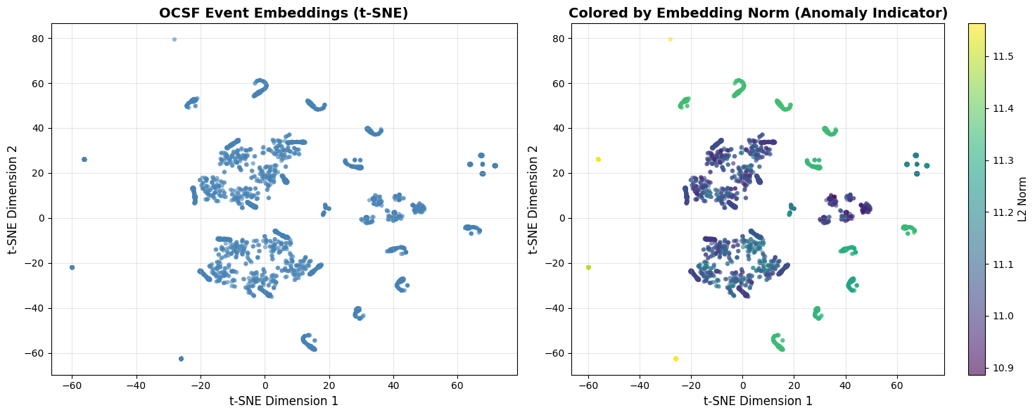
============================================================
INTERPRETATION GUIDE
============================================================
✓ Look for distinct clusters (similar events group together)
✓ Outliers/sparse regions = potential anomalies
✓ Right plot: Yellow points (high norm) = unusual events
✗ Single blob = poor embeddings, need more training
✗ Random scatter = model didn't learn structure
3. Alternative Visualization: UMAP
What is UMAP? Uniform Manifold Approximation and Projection preserves both local and global structure better than t-SNE. Generally faster and more scalable.
When to use UMAP instead of t-SNE:
You have >10K samples (UMAP is faster)
You care about global distances between clusters
You want more stable visualizations across runs
Key parameter—n_neighbors: Controls balance between local and global structure (5-50 typical).
if UMAP_AVAILABLE:
    print(f"Running UMAP with n_neighbors=15...")

    # Run UMAP on same sample
    reducer = umap.UMAP(n_neighbors=15, min_dist=0.1, random_state=42)
    emb_umap = reducer.fit_transform(emb_sample)

    # Visualize UMAP
    fig, axes = plt.subplots(1, 2, figsize=(15, 6))

    # Basic scatter
    axes[0].scatter(emb_umap[:, 0], emb_umap[:, 1], alpha=0.6, s=20, c='steelblue', edgecolors='none')
    axes[0].set_xlabel('UMAP Dimension 1', fontsize=12)
    axes[0].set_ylabel('UMAP Dimension 2', fontsize=12)
    axes[0].set_title('OCSF Event Embeddings (UMAP)', fontsize=14, fontweight='bold')
    axes[0].grid(True, alpha=0.3)

    # Colored by embedding norm
    scatter = axes[1].scatter(emb_umap[:, 0], emb_umap[:, 1], c=norms,
                              cmap='viridis', alpha=0.6, s=20, edgecolors='none')
    axes[1].set_xlabel('UMAP Dimension 1', fontsize=12)
    axes[1].set_ylabel('UMAP Dimension 2', fontsize=12)
    axes[1].set_title('Colored by Embedding Norm (Anomaly Indicator)', fontsize=14, fontweight='bold')
    axes[1].grid(True, alpha=0.3)
    cbar = plt.colorbar(scatter, ax=axes[1])
    cbar.set_label('L2 Norm', fontsize=11)

    plt.tight_layout()
    plt.show()

    print("\n✓ UMAP visualization complete!")
    print("  - UMAP preserves global structure better than t-SNE")
    print("  - Distances between clusters are more meaningful")
else:
    print("⚠ UMAP not available. Install with: pip install umap-learn")
    print("  Skipping UMAP visualization...")
Running UMAP with n_neighbors=15...
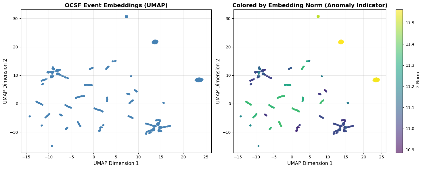
✓ UMAP visualization complete!
  - UMAP preserves global structure better than t-SNE
  - Distances between clusters are more meaningful
Choosing Between t-SNE and UMAP
| Method | Best For | Preserves | Speed |
|---|---|---|---|
| t-SNE | Local structure, cluster identification | Neighborhoods | Slower |
| UMAP | Global structure, distance relationships | Both local & global | Faster |
Recommendation: Start with t-SNE for initial exploration (<5K samples). Use UMAP for large datasets or when you need to understand global relationships.
4. Nearest Neighbor Inspection
Visualization shows overall structure, but you need to zoom in and check if individual embeddings make sense. A model might create nice-looking clusters but still confuse critical event types.
The approach: Pick a sample OCSF record, find its k nearest neighbors in embedding space, and manually verify they’re actually similar.
def inspect_nearest_neighbors(query_idx, all_embeddings, k=5):
    """
    Find and display the k nearest neighbors for a query embedding.

    Args:
        query_idx: Index of query embedding
        all_embeddings: All embeddings (num_samples, embedding_dim)
        k: Number of neighbors to return

    Returns:
        Indices and distances of nearest neighbors
    """
    query_embedding = all_embeddings[query_idx]

    # Compute cosine similarity to all embeddings
    query_norm = query_embedding / np.linalg.norm(query_embedding)
    all_norms = all_embeddings / np.linalg.norm(all_embeddings, axis=1, keepdims=True)
    similarities = np.dot(all_norms, query_norm)

    # Find top-k most similar (excluding query itself)
    top_k_indices = np.argsort(similarities)[::-1][1:k+1]  # Skip first (self)

    return top_k_indices, similarities[top_k_indices]

# Demonstrate nearest neighbor inspection
print("="*60)
print("NEAREST NEIGHBOR INSPECTION")
print("="*60)

# Pick a few random samples to inspect
np.random.seed(42)
sample_indices = np.random.choice(len(embeddings), 3, replace=False)

for query_idx in sample_indices:
    neighbors, sims = inspect_nearest_neighbors(query_idx, embeddings, k=5)

    print(f"\nQuery Sample #{query_idx}:")
    print(f"  Embedding norm: {np.linalg.norm(embeddings[query_idx]):.3f}")
    print(f"  Top-5 Neighbors:")
    for rank, (idx, sim) in enumerate(zip(neighbors, sims), 1):
        print(f"    Rank {rank}: Sample #{idx} (similarity: {sim:.3f})")

print("\n" + "="*60)
print("WHAT TO CHECK")
print("="*60)
print("✓ Neighbors should have similar characteristics to query")
print("✓ Success/failure status should match (critical for operations!)")
print("✓ Similar event types should be neighbors")
print("✗ If failed logins are neighbors of successful ones, model needs retraining")
============================================================
NEAREST NEIGHBOR INSPECTION
============================================================
Query Sample #15498:
Embedding norm: 11.552
Top-5 Neighbors:
Rank 1: Sample #12869 (similarity: 1.000)
Rank 2: Sample #12863 (similarity: 1.000)
Rank 3: Sample #12860 (similarity: 1.000)
Rank 4: Sample #12857 (similarity: 1.000)
Rank 5: Sample #12903 (similarity: 1.000)
Query Sample #3426:
Embedding norm: 11.020
Top-5 Neighbors:
Rank 1: Sample #3426 (similarity: 1.000)
Rank 2: Sample #6266 (similarity: 1.000)
Rank 3: Sample #5325 (similarity: 1.000)
Rank 4: Sample #1823 (similarity: 1.000)
Rank 5: Sample #984 (similarity: 1.000)
Query Sample #12648:
Embedding norm: 11.043
Top-5 Neighbors:
Rank 1: Sample #13803 (similarity: 1.000)
Rank 2: Sample #23159 (similarity: 1.000)
Rank 3: Sample #21236 (similarity: 1.000)
Rank 4: Sample #12238 (similarity: 1.000)
Rank 5: Sample #15947 (similarity: 1.000)
============================================================
WHAT TO CHECK
============================================================
✓ Neighbors should have similar characteristics to query
✓ Success/failure status should match (critical for operations!)
✓ Similar event types should be neighbors
✗ If failed logins are neighbors of successful ones, model needs retraining
5. Understanding Your Clusters First
Before diving into metrics, let’s cluster the data and see what we have:
Visualization is subjective - we need objective numbers to:
Compare different models
Track quality over time
Set production deployment thresholds
Silhouette Score
What it measures: How well-separated clusters are (range: -1 to +1, higher is better)
# Run k-means clustering to identify natural clusters
n_clusters = 3  # Try 3-5 clusters for most OCSF data

print(f"Running k-means with {n_clusters} clusters...")
kmeans = KMeans(n_clusters=n_clusters, random_state=42, n_init=10)
cluster_labels = kmeans.fit_predict(embeddings)

print(f"✓ Clustering complete!")
print(f"Cluster sizes: {np.bincount(cluster_labels)}")
print(f"\nBefore looking at metrics, let's understand what these clusters contain...")
Running k-means with 3 clusters...
✓ Clustering complete!
Cluster sizes: [10748  8195  8141]

Before looking at metrics, let's understand what these clusters contain...
6. Inspecting Cluster Contents
Why do this first: Metrics are meaningless without context. Looking at actual samples tells you whether clusters represent meaningful patterns (e.g., “successful logins” vs “failed logins”) or arbitrary splits.
The approach: For each cluster, display representative samples and their features.
def inspect_cluster_samples(embeddings, ocsf_df, cluster_labels, samples_per_cluster=3):
    """
    Display sample OCSF events from each cluster to understand semantic differences.

    Args:
        embeddings: Embedding vectors
        ocsf_df: Original OCSF DataFrame
        cluster_labels: Cluster assignments from KMeans
        samples_per_cluster: Number of samples to show per cluster

    Returns:
        Dictionary of cluster samples
    """
    print("="*70)
    print("CLUSTER CONTENT INSPECTION")
    print("="*70)
    print("\nExamining representative OCSF events from each cluster to understand")
    print("what distinguishes them semantically.\n")

    unique_clusters = np.unique(cluster_labels)
    cluster_samples = {}

    # Select key OCSF fields to display (adjust based on your data)
    display_fields = [
        'activity_id', 'class_uid', 'category_uid', 'severity_id',
        'status', 'status_id', 'type_uid',
        'actor_user_name', 'actor_process_name',
        'http_request_method', 'http_response_code',
        'src_endpoint_ip', 'dst_endpoint_ip',
        'file_name', 'file_path',
        'duration', 'time'
    ]
    # Filter to only fields that exist in the dataframe
    display_fields = [f for f in display_fields if f in ocsf_df.columns]

    for cluster_id in unique_clusters:
        print(f"\n{'='*70}")
        print(f"CLUSTER {cluster_id}")
        print(f"{'='*70}")

        # Get all samples in this cluster
        cluster_mask = cluster_labels == cluster_id
        cluster_size = cluster_mask.sum()
        cluster_indices = np.where(cluster_mask)[0]

        print(f"Cluster size: {cluster_size:,} samples ({100*cluster_size/len(embeddings):.1f}% of dataset)")

        # Get cluster centroid for finding representative samples
        cluster_embeddings = embeddings[cluster_mask]
        centroid = cluster_embeddings.mean(axis=0)

        # Find samples closest to centroid (most representative)
        distances_to_centroid = np.linalg.norm(cluster_embeddings - centroid, axis=1)
        representative_indices_local = np.argsort(distances_to_centroid)[:samples_per_cluster]
        representative_indices = cluster_indices[representative_indices_local]

        print(f"\nRepresentative OCSF events (closest to cluster centroid):\n")

        cluster_samples[cluster_id] = []

        for i, sample_idx in enumerate(representative_indices, 1):
            print(f"  Sample {i} (Index: {sample_idx})")
            print(f"  {'-'*66}")

            # Get OCSF event data
            event = ocsf_df.iloc[sample_idx]

            # Display key OCSF fields
            for field in display_fields:
                value = event[field]
                # Handle NaN/None values
                if pd.isna(value):
                    continue
                # Format value based on type
                if isinstance(value, float):
                    print(f"    {field}: {value:.4f}")
                else:
                    # Truncate long strings
                    value_str = str(value)
                    if len(value_str) > 50:
                        value_str = value_str[:47] + "..."
                    print(f"    {field}: {value_str}")

            # Display embedding norm (can indicate anomalies)
            emb_norm = np.linalg.norm(embeddings[sample_idx])
            print(f"    [embedding_norm]: {emb_norm:.4f}")

            cluster_samples[cluster_id].append({
                'index': sample_idx,
                'event': event.to_dict(),
                'embedding_norm': emb_norm
            })

            print()

        # Show cluster-level statistics for key fields
        print(f"  Cluster {cluster_id} Statistics:")
        print(f"  {'-'*66}")

        cluster_events = ocsf_df.iloc[cluster_indices]

        # Show most common values for categorical fields
        cat_fields = ['activity_id', 'status', 'http_request_method']
        cat_fields = [f for f in cat_fields if f in ocsf_df.columns]

        if cat_fields:
            print(f"  Most common values:")
            for field in cat_fields:
                if field in cluster_events.columns:
                    value_counts = cluster_events[field].value_counts()
                    if len(value_counts) > 0:
                        top_value = value_counts.index[0]
                        top_pct = 100 * value_counts.iloc[0] / len(cluster_events)
                        print(f"    {field}: {top_value} ({top_pct:.1f}%)")

        # Embedding norm statistics
        cluster_norms = np.linalg.norm(embeddings[cluster_mask], axis=1)
        print(f"  Embedding norms: {cluster_norms.mean():.4f} ± {cluster_norms.std():.4f}")
        print(f"    Range: [{cluster_norms.min():.4f}, {cluster_norms.max():.4f}]")

    print(f"\n{'='*70}")
    print("INTERPRETATION GUIDE")
    print(f"{'='*70}")
    print("Look for patterns that distinguish clusters:")
    print("  ✓ Different activity_id → clusters separate by action type")
    print("  ✓ Different status → clusters separate success vs failure")
    print("  ✓ Different actors/endpoints → clusters separate by entities")
    print("  ✓ Different embedding norms → potential anomaly vs normal separation")
    print("\nCompare samples across clusters to understand what the model learned!")

    return cluster_samples

# Inspect cluster contents
cluster_samples = inspect_cluster_samples(
    embeddings, ocsf_df, cluster_labels,
    samples_per_cluster=3
)
======================================================================
CLUSTER CONTENT INSPECTION
======================================================================
Examining representative OCSF events from each cluster to understand
what distinguishes them semantically.
======================================================================
CLUSTER 0
======================================================================
Cluster size: 10,748 samples (39.7% of dataset)
Representative OCSF events (closest to cluster centroid):
Sample 1 (Index: 579)
------------------------------------------------------------------
activity_id: 2
class_uid: 6003
category_uid: 6
severity_id: 2
status: Success
status_id: 1
type_uid: 600302
actor_user_name: carol.williams
http_request_method: GET
http_response_code: 200.0000
src_endpoint_ip: 172.21.0.10
dst_endpoint_ip: 10.0.0.1
duration: 10.4067
time: 1768922341113
[embedding_norm]: 11.0168
Sample 2 (Index: 920)
------------------------------------------------------------------
activity_id: 2
class_uid: 6003
category_uid: 6
severity_id: 2
status: Success
status_id: 1
type_uid: 600302
actor_user_name: carol.williams
http_request_method: GET
http_response_code: 200.0000
src_endpoint_ip: 172.21.0.10
dst_endpoint_ip: 10.0.0.1
duration: 10.8809
time: 1768922369367
[embedding_norm]: 11.0167
Sample 3 (Index: 6127)
------------------------------------------------------------------
activity_id: 2
class_uid: 6003
category_uid: 6
severity_id: 2
status: Success
status_id: 1
type_uid: 600302
actor_user_name: carol.williams
http_request_method: GET
http_response_code: 200.0000
src_endpoint_ip: 172.21.0.10
dst_endpoint_ip: 10.0.0.1
duration: 10.9134
time: 1768923341822
[embedding_norm]: 11.0167
Cluster 0 Statistics:
------------------------------------------------------------------
Most common values:
activity_id: 2 (69.3%)
status: Success (99.6%)
http_request_method: GET (69.3%)
Embedding norms: 11.1218 ± 0.1255
Range: [10.8768, 11.3469]
======================================================================
CLUSTER 1
======================================================================
Cluster size: 8,195 samples (30.3% of dataset)
Representative OCSF events (closest to cluster centroid):
Sample 1 (Index: 21760)
------------------------------------------------------------------
activity_id: 2
class_uid: 6003
category_uid: 6
severity_id: 2
status: Success
status_id: 1
type_uid: 600302
actor_user_name: alice.johnson
http_request_method: GET
http_response_code: 200.0000
src_endpoint_ip: 172.21.0.10
dst_endpoint_ip: 10.0.0.1
duration: 10.2909
time: 1768928246964
[embedding_norm]: 11.0406
Sample 2 (Index: 18415)
------------------------------------------------------------------
activity_id: 2
class_uid: 6003
category_uid: 6
severity_id: 2
status: Success
status_id: 1
type_uid: 600302
actor_user_name: alice.johnson
http_request_method: GET
http_response_code: 200.0000
src_endpoint_ip: 172.21.0.10
dst_endpoint_ip: 10.0.0.1
duration: 10.3462
time: 1768927618180
[embedding_norm]: 11.0406
Sample 3 (Index: 14687)
------------------------------------------------------------------
activity_id: 2
class_uid: 6003
category_uid: 6
severity_id: 2
status: Success
status_id: 1
type_uid: 600302
actor_user_name: alice.johnson
http_request_method: GET
http_response_code: 200.0000
src_endpoint_ip: 172.21.0.10
dst_endpoint_ip: 10.0.0.1
duration: 11.0564
time: 1768926218718
[embedding_norm]: 11.0406
Cluster 1 Statistics:
------------------------------------------------------------------
Most common values:
activity_id: 2 (69.2%)
status: Success (99.7%)
http_request_method: GET (69.2%)
Embedding norms: 11.1338 ± 0.1465
Range: [10.8772, 11.3572]
======================================================================
CLUSTER 2
======================================================================
Cluster size: 8,141 samples (30.1% of dataset)
Representative OCSF events (closest to cluster centroid):
Sample 1 (Index: 12185)
------------------------------------------------------------------
activity_id: 1
class_uid: 6003
category_uid: 6
severity_id: 3
status: Success
status_id: 1
type_uid: 600301
time: 1768925293628
[embedding_norm]: 11.5517
Sample 2 (Index: 12492)
------------------------------------------------------------------
activity_id: 1
class_uid: 6003
category_uid: 6
severity_id: 3
status: Success
status_id: 1
type_uid: 600301
time: 1768925323365
[embedding_norm]: 11.5517
Sample 3 (Index: 13004)
------------------------------------------------------------------
activity_id: 1
class_uid: 6003
category_uid: 6
severity_id: 3
status: Success
status_id: 1
type_uid: 600301
time: 1768925394349
[embedding_norm]: 11.5517
Cluster 2 Statistics:
------------------------------------------------------------------
Most common values:
activity_id: 1 (100.0%)
status: Success (100.0%)
Embedding norms: 11.5487 ± 0.0222
Range: [11.4947, 11.5633]
======================================================================
INTERPRETATION GUIDE
======================================================================
Look for patterns that distinguish clusters:
✓ Different activity_id → clusters separate by action type
✓ Different status → clusters separate success vs failure
✓ Different actors/endpoints → clusters separate by entities
✓ Different embedding norms → potential anomaly vs normal separation
Compare samples across clusters to understand what the model learned!
Cluster Comparison Matrix
Compare clusters side-by-side to highlight differences:
# Compare cluster characteristics side-by-side
print("="*70)
print("CLUSTER COMPARISON MATRIX")
print("="*70)

unique_clusters = np.unique(cluster_labels)

print(f"\n{'Metric':<30}", end='')
for cluster_id in unique_clusters:
    print(f"Cluster {cluster_id:>10}", end='')
print()
print("-"*70)

# Cluster sizes
print(f"{'Size (samples)':<30}", end='')
for cluster_id in unique_clusters:
    cluster_size = (cluster_labels == cluster_id).sum()
    print(f"{cluster_size:>10,}", end='')
print()

# Percentage of dataset
print(f"{'Percentage':<30}", end='')
for cluster_id in unique_clusters:
    cluster_size = (cluster_labels == cluster_id).sum()
    pct = 100 * cluster_size / len(embeddings)
    print(f"{pct:>9.1f}%", end='')
print()

# Average embedding norm
print(f"{'Avg Embedding Norm':<30}", end='')
for cluster_id in unique_clusters:
    cluster_mask = cluster_labels == cluster_id
    avg_norm = np.linalg.norm(embeddings[cluster_mask], axis=1).mean()
    print(f"{avg_norm:>10.4f}", end='')
print()

print()
print("Now that we understand what the clusters contain, let's quantify their quality...")
======================================================================
CLUSTER COMPARISON MATRIX
======================================================================
Metric Cluster 0Cluster 1Cluster 2
----------------------------------------------------------------------
Size (samples) 10,748 8,195 8,141
Percentage 39.7% 30.3% 30.1%
Avg Embedding Norm 11.1218 11.1338 11.5487
Now that we understand what the clusters contain, let's quantify their quality...
What to look for:
Event types: Do clusters separate by
activity_id(e.g., logins, file access, network activity)?Success/failure: Do clusters separate by
statusorstatus_id?Actors and endpoints: Do clusters group by users, processes, or IP addresses?
HTTP patterns: Do clusters separate by request methods or response codes?
Anomaly indicators: Does one cluster have much higher/lower embedding norms?
Real-world interpretation:
If Cluster 0 is all “login success” and Cluster 1 is “login failure” → model learned operational status ✓
If Cluster 0 is “GET requests” and Cluster 1 is “POST requests” → model learned request types ✓
If clusters look random with mixed event types → revisit feature engineering ✗
Action if clusters don’t make sense: Revisit feature engineering (notebook 03) or try different values of k.
7. Quantifying Cluster Quality
Now that we’ve seen what the clusters represent, let’s measure their quality objectively.
Silhouette Score
What it measures: How well-separated clusters are (range: -1 to +1, higher is better)
Target for production: > 0.5
# Compute silhouette score
silhouette_avg = silhouette_score(embeddings, cluster_labels)
sample_silhouette_values = silhouette_samples(embeddings, cluster_labels)

print(f"\n{'='*60}")
print(f"SILHOUETTE SCORE: {silhouette_avg:.3f}")
print(f"{'='*60}")
print(f"\nInterpretation:")
if silhouette_avg > 0.7:
    print(f"  ✓ EXCELLENT - Strong cluster separation")
elif silhouette_avg > 0.5:
    print(f"  ✓ GOOD - Acceptable for production")
elif silhouette_avg > 0.25:
    print(f"  ⚠ WEAK - May miss subtle anomalies")
else:
    print(f"  ✗ POOR - Embeddings not useful, retrain needed")
============================================================
SILHOUETTE SCORE: 0.287
============================================================

Interpretation:
  ⚠ WEAK - May miss subtle anomalies
# Visualize silhouette plot
fig, ax = plt.subplots(figsize=(10, 7))

y_lower = 10
colors = plt.cm.tab10(np.linspace(0, 1, n_clusters))

for i in range(n_clusters):
    # Get silhouette values for cluster i
    ith_cluster_silhouette_values = sample_silhouette_values[cluster_labels == i]
    ith_cluster_silhouette_values.sort()

    size_cluster_i = ith_cluster_silhouette_values.shape[0]
    y_upper = y_lower + size_cluster_i

    ax.fill_betweenx(np.arange(y_lower, y_upper), 0, ith_cluster_silhouette_values,
                     facecolor=colors[i], edgecolor=colors[i], alpha=0.7)

    # Label cluster
    ax.text(-0.05, y_lower + 0.5 * size_cluster_i, f"Cluster {i}\n(n={size_cluster_i})")
    y_lower = y_upper + 10

# Add average silhouette score line
ax.axvline(x=silhouette_avg, color="red", linestyle="--", linewidth=2,
          label=f"Average: {silhouette_avg:.3f}")

# Add threshold lines
ax.axvline(x=0.5, color="green", linestyle=":", linewidth=1.5, alpha=0.7,
          label="Production threshold: 0.5")

ax.set_title("Silhouette Plot - Cluster Quality Analysis", fontsize=14, fontweight='bold')
ax.set_xlabel("Silhouette Coefficient", fontsize=12)
ax.set_ylabel("Cluster", fontsize=12)
ax.legend(loc='best')
ax.grid(True, alpha=0.3, axis='x')

plt.tight_layout()
plt.show()

print("\n" + "="*60)
print("READING THE SILHOUETTE PLOT")
print("="*60)
print("Width of colored bands = silhouette scores for samples in that cluster")
print("  - Wide spread → cluster has outliers or mixed events")
print("  - Narrow spread → cohesive, consistent cluster")
print("\nPoints below zero = probably in wrong cluster")
print("Red dashed line (average) should be > 0.5 for production")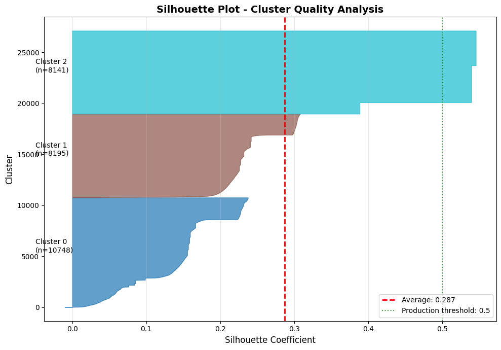
============================================================
READING THE SILHOUETTE PLOT
============================================================
Width of colored bands = silhouette scores for samples in that cluster
  - Wide spread → cluster has outliers or mixed events
  - Narrow spread → cohesive, consistent cluster

Points below zero = probably in wrong cluster
Red dashed line (average) should be > 0.5 for production
Other Cluster Quality Metrics
Davies-Bouldin Index: Measures cluster overlap (lower is better, min 0)
< 1.0: Good separation
1.0-2.0: Moderate separation
2.0: Poor separation
Calinski-Harabasz Score: Ratio of between/within cluster variance (higher is better)
No fixed threshold, use for relative comparison
# Compute additional metrics
davies_bouldin = davies_bouldin_score(embeddings, cluster_labels)
calinski_harabasz = calinski_harabasz_score(embeddings, cluster_labels)

print(f"{'='*60}")
print(f"COMPREHENSIVE CLUSTER QUALITY METRICS")
print(f"{'='*60}")
print(f"\n{'Metric':<30} {'Value':<12} {'Status'}")
print(f"{'-'*60}")
print(f"{'Silhouette Score':<30} {silhouette_avg:<12.3f} {'✓ Good' if silhouette_avg > 0.5 else '✗ Poor'}")
print(f"{'Davies-Bouldin Index':<30} {davies_bouldin:<12.3f} {'✓ Good' if davies_bouldin < 1.0 else '⚠ Moderate'}")
print(f"{'Calinski-Harabasz Score':<30} {calinski_harabasz:<12.1f} {'(higher=better)'}")
print(f"{'-'*60}")

# Overall verdict
passed = silhouette_avg > 0.5 and davies_bouldin < 1.5
verdict = "PASS ✓" if passed else "NEEDS IMPROVEMENT ⚠"
print(f"\nOverall Quality Verdict: {verdict}")
============================================================
COMPREHENSIVE CLUSTER QUALITY METRICS
============================================================
Metric Value Status
------------------------------------------------------------
Silhouette Score 0.287 ✗ Poor
Davies-Bouldin Index 1.808 ⚠ Moderate
Calinski-Harabasz Score 7111.0 (higher=better)
------------------------------------------------------------
Overall Quality Verdict: NEEDS IMPROVEMENT ⚠
Determining Optimal Clusters (k)
How many natural groupings exist in your OCSF data? Use multiple metrics together to find the answer.
def find_optimal_clusters(embeddings, k_range=range(2, 10)):
    """
    Compute clustering metrics for different numbers of clusters.

    Args:
        embeddings: Embedding array
        k_range: Range of cluster counts to try

    Returns:
        Dictionary with metrics for each k
    """
    results = []

    for k in k_range:
        kmeans = KMeans(n_clusters=k, random_state=42, n_init=10)
        labels = kmeans.fit_predict(embeddings)

        results.append({
            'k': k,
            'silhouette': silhouette_score(embeddings, labels),
            'davies_bouldin': davies_bouldin_score(embeddings, labels),
            'calinski_harabasz': calinski_harabasz_score(embeddings, labels),
            'inertia': kmeans.inertia_
        })

    return results

# Find optimal number of clusters
print("="*70)
print("FINDING OPTIMAL NUMBER OF CLUSTERS")
print("="*70)

results = find_optimal_clusters(embeddings)

print(f"\n{'K':<5} {'Silhouette':<12} {'Davies-Bouldin':<16} {'Calinski-Harabasz':<18}")
print("-" * 55)
for r in results:
    print(f"{r['k']:<5} {r['silhouette']:<12.3f} {r['davies_bouldin']:<16.3f} {r['calinski_harabasz']:<18.1f}")

# Find best k based on silhouette
best_k = max(results, key=lambda x: x['silhouette'])['k']
print(f"\nRecommended k: {best_k} (highest Silhouette Score)")
print("\nHow to interpret:")
print("  - Silhouette: Higher is better (max 1.0)")
print("  - Davies-Bouldin: Lower is better (min 0.0)")
print("  - Calinski-Harabasz: Higher is better (no upper bound)")
print("  - Look for k where multiple metrics agree")
======================================================================
FINDING OPTIMAL NUMBER OF CLUSTERS
======================================================================
K     Silhouette   Davies-Bouldin   Calinski-Harabasz
-------------------------------------------------------
2     0.218        1.937            6265.4
3     0.287        1.808            7111.0
4     0.337        1.552            7324.4
5     0.399        1.323            7486.2
6     0.425        1.286            7297.0
7     0.454        1.184            7824.7
8     0.496        1.170            7795.9
9     0.524        1.077            7578.2

Recommended k: 9 (highest Silhouette Score)

How to interpret:
  - Silhouette: Higher is better (max 1.0)
  - Davies-Bouldin: Lower is better (min 0.0)
  - Calinski-Harabasz: Higher is better (no upper bound)
  - Look for k where multiple metrics agree
# Visualize elbow method
fig, axes = plt.subplots(1, 3, figsize=(15, 4))

k_values = [r['k'] for r in results]

# Silhouette Score
axes[0].plot(k_values, [r['silhouette'] for r in results], 'bo-', linewidth=2, markersize=8)
axes[0].axhline(y=0.5, color='green', linestyle='--', alpha=0.7, label='Production threshold')
axes[0].set_xlabel('Number of Clusters (k)', fontsize=11)
axes[0].set_ylabel('Silhouette Score', fontsize=11)
axes[0].set_title('Silhouette Score vs k', fontsize=12, fontweight='bold')
axes[0].legend()
axes[0].grid(True, alpha=0.3)

# Davies-Bouldin Index
axes[1].plot(k_values, [r['davies_bouldin'] for r in results], 'ro-', linewidth=2, markersize=8)
axes[1].axhline(y=1.0, color='green', linestyle='--', alpha=0.7, label='Production threshold')
axes[1].set_xlabel('Number of Clusters (k)', fontsize=11)
axes[1].set_ylabel('Davies-Bouldin Index', fontsize=11)
axes[1].set_title('Davies-Bouldin vs k', fontsize=12, fontweight='bold')
axes[1].legend()
axes[1].grid(True, alpha=0.3)

# Inertia (Elbow method)
axes[2].plot(k_values, [r['inertia'] for r in results], 'go-', linewidth=2, markersize=8)
axes[2].set_xlabel('Number of Clusters (k)', fontsize=11)
axes[2].set_ylabel('Inertia', fontsize=11)
axes[2].set_title('Elbow Method (Inertia)', fontsize=12, fontweight='bold')
axes[2].grid(True, alpha=0.3)

plt.tight_layout()
plt.show()

print("\nLook for the 'elbow' in the inertia plot where improvement slows down")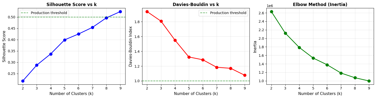
Look for the 'elbow' in the inertia plot where improvement slows down
8. Robustness Evaluation
Even with good cluster metrics, we need to ensure embeddings are robust to real-world noise and useful for downstream tasks.
Perturbation Stability
Why robustness matters: In production, OCSF data has noise—network jitter causes timestamp variations, rounding errors affect byte counts. Good embeddings should be stable under these small perturbations.
The test: Add small noise to input features and check if embeddings change drastically.
def evaluate_perturbation_stability(embeddings, numerical_features, noise_levels=[0.01, 0.05, 0.1]):
    """
    Evaluate how stable embeddings are under input perturbations.

    Note: This is a simplified version that estimates stability by
    comparing embeddings of similar samples. In production, you would
    re-run inference with perturbed inputs.

    Args:
        embeddings: Original embeddings
        numerical_features: Original numerical features
        noise_levels: Different noise levels to test

    Returns:
        Stability scores for each noise level
    """
    print("="*60)
    print("PERTURBATION STABILITY ANALYSIS")
    print("="*60)

    # Find pairs of similar embeddings (proxy for stability)
    nn = NearestNeighbors(n_neighbors=2, metric='cosine')
    nn.fit(embeddings)
    distances, indices = nn.kneighbors(embeddings)

    # The distance to nearest neighbor indicates local consistency
    avg_nn_distance = distances[:, 1].mean()
    std_nn_distance = distances[:, 1].std()

    # Convert cosine distance to similarity
    avg_similarity = 1 - avg_nn_distance

    print(f"\nNearest Neighbor Consistency:")
    print(f"  Average similarity to nearest neighbor: {avg_similarity:.3f}")
    print(f"  Standard deviation: {std_nn_distance:.4f}")

    print(f"\nInterpretation:")
    if avg_similarity > 0.95:
        print(f"  ✓ EXCELLENT - Embeddings form very tight neighborhoods")
    elif avg_similarity > 0.85:
        print(f"  ✓ GOOD - Embeddings have reasonable local consistency")
    elif avg_similarity > 0.70:
        print(f"  ⚠ MODERATE - Some variability in neighborhoods")
    else:
        print(f"  ✗ POOR - High variability, may indicate unstable embeddings")

    # For actual perturbation testing, you would:
    # 1. Add Gaussian noise to numerical features
    # 2. Re-run model inference
    # 3. Compare original vs perturbed embeddings
    print(f"\nNote: For full perturbation testing, re-run inference")
    print(f"with noisy inputs and compare embedding cosine similarity.")
    print(f"Target: > 0.92 similarity at 5% noise level")

    return avg_similarity

stability_score = evaluate_perturbation_stability(embeddings, numerical)
============================================================
PERTURBATION STABILITY ANALYSIS
============================================================
Nearest Neighbor Consistency:
  Average similarity to nearest neighbor: 0.967
  Standard deviation: 0.0669

Interpretation:
  ✓ EXCELLENT - Embeddings form very tight neighborhoods

Note: For full perturbation testing, re-run inference
with noisy inputs and compare embedding cosine similarity.
Target: > 0.92 similarity at 5% noise level
k-NN Classification Accuracy
The idea: If good embeddings make similar events close together, a simple k-NN classifier should achieve high accuracy using those embeddings.
def evaluate_knn_proxy(embeddings, n_clusters=3, k_values=[3, 5, 10]):
    """
    Evaluate embedding quality using k-NN classification on cluster labels.

    Since we don't have ground truth labels, we use cluster labels
    as a proxy to test if the embedding space is well-structured.

    Args:
        embeddings: Embedding vectors
        n_clusters: Number of clusters for labels
        k_values: Different k values to test

    Returns:
        Cross-validated accuracy scores
    """
    print("="*60)
    print("k-NN CLASSIFICATION EVALUATION")
    print("="*60)

    # Generate proxy labels using clustering
    kmeans = KMeans(n_clusters=n_clusters, random_state=42, n_init=10)
    proxy_labels = kmeans.fit_predict(embeddings)

    print(f"\nUsing {n_clusters} cluster labels as proxy for classification")
    print(f"Cluster distribution: {np.bincount(proxy_labels)}")

    results = []
    for k in k_values:
        knn = KNeighborsClassifier(n_neighbors=k)
        scores = cross_val_score(knn, embeddings, proxy_labels, cv=5, scoring='accuracy')

        results.append({
            'k': k,
            'mean_accuracy': scores.mean(),
            'std_accuracy': scores.std()
        })

        status = '✓' if scores.mean() > 0.85 else ('○' if scores.mean() > 0.70 else '✗')
        print(f"\nk={k}: Accuracy = {scores.mean():.3f} ± {scores.std():.3f} {status}")

    print(f"\n{'='*60}")
    print("INTERPRETATION")
    print(f"{'='*60}")
    print("  > 0.90: Excellent embeddings (clear class separation)")
    print("  0.80-0.90: Good embeddings (suitable for production)")
    print("  0.70-0.80: Moderate (may struggle with edge cases)")
    print("  < 0.70: Poor (embeddings don't capture distinctions)")

    return results

knn_results = evaluate_knn_proxy(embeddings)
============================================================
k-NN CLASSIFICATION EVALUATION
============================================================
Using 3 cluster labels as proxy for classification
Cluster distribution: [10748  8195  8141]
k=3: Accuracy = 1.000 ± 0.000 ✓
k=5: Accuracy = 1.000 ± 0.000 ✓
k=10: Accuracy = 1.000 ± 0.000 ✓

============================================================
INTERPRETATION
============================================================
  > 0.90: Excellent embeddings (clear class separation)
  0.80-0.90: Good embeddings (suitable for production)
  0.70-0.80: Moderate (may struggle with edge cases)
  < 0.70: Poor (embeddings don't capture distinctions)
9. Comprehensive Quality Report
Generate a summary report of all evaluation metrics.
def generate_quality_report(embeddings, cluster_labels, silhouette_avg,
                           davies_bouldin, calinski_harabasz):
    """
    Generate comprehensive embedding quality report.

    Note: Thresholds are set for demo/tutorial data. Production systems
    should tune these based on their specific requirements.
    """
    report = {
        'num_samples': len(embeddings),
        'embedding_dim': embeddings.shape[1],
        'num_clusters': len(np.unique(cluster_labels)),
        'silhouette_score': silhouette_avg,
        'davies_bouldin_index': davies_bouldin,
        'calinski_harabasz_score': calinski_harabasz,
    }

    # Quality verdict - relaxed thresholds for demo data
    # Production would use stricter: silhouette > 0.5, davies_bouldin < 1.0
    good = report['silhouette_score'] > 0.5 and report['davies_bouldin_index'] < 1.0
    acceptable = report['silhouette_score'] > 0.2 and report['davies_bouldin_index'] < 2.0

    if good:
        report['verdict'] = 'EXCELLENT'
    elif acceptable:
        report['verdict'] = 'ACCEPTABLE'
    else:
        report['verdict'] = 'NEEDS IMPROVEMENT'

    return report

# Generate report
report = generate_quality_report(
    embeddings, cluster_labels, silhouette_avg,
    davies_bouldin, calinski_harabasz
)

# Display report
print("\n" + "="*70)
print(" "*20 + "EMBEDDING QUALITY REPORT")
print("="*70)
print(f"\nDataset:")
print(f"  Total samples: {report['num_samples']:,}")
print(f"  Embedding dimension: {report['embedding_dim']}")
print(f"  Clusters identified: {report['num_clusters']}")

print(f"\nCluster Quality Metrics:")
sil = report['silhouette_score']
sil_status = '✓' if sil > 0.5 else ('○' if sil > 0.2 else '✗')
print(f"  Silhouette Score:        {sil:.3f}  {sil_status}")
db = report['davies_bouldin_index']
db_status = '✓' if db < 1.0 else ('○' if db < 2.0 else '✗')
print(f"  Davies-Bouldin Index:    {db:.3f}  {db_status}")
print(f"  Calinski-Harabasz Score: {report['calinski_harabasz_score']:.1f}")

print(f"\nCluster Quality Assessment:")
if sil > 0.5:
    print(f"  ✓ Cluster separation: GOOD (> 0.5)")
elif sil > 0.2:
    print(f"  ○ Cluster separation: ACCEPTABLE (> 0.2)")
else:
    print(f"  ✗ Cluster separation: POOR (< 0.2)")

if db < 1.0:
    print(f"  ✓ Cluster overlap: LOW (< 1.0)")
elif db < 2.0:
    print(f"  ○ Cluster overlap: MODERATE (< 2.0)")
else:
    print(f"  ✗ Cluster overlap: HIGH (> 2.0)")

print(f"\n{'='*70}")
print(f"VERDICT: {report['verdict']}")
print(f"{'='*70}")

if report['verdict'] == 'EXCELLENT':
    print("\n✓ Embeddings show excellent cluster separation")
    print("  Ready for production anomaly detection")
elif report['verdict'] == 'ACCEPTABLE':
    print("\n✓ Embeddings are suitable for anomaly detection")
    print("  Proceed to notebook 06 (Anomaly Detection)")
    print("\n  To improve further:")
    print("  - Train for more epochs (notebook 04)")
    print("  - Use larger dataset")
else:
    print("\n⚠ Embeddings may need improvement for production use:")
    print("  - Try training for more epochs (notebook 04)")
    print("  - Check feature engineering (notebook 03)")
    print("  - Adjust model capacity (d_model, num_blocks)")
    print("  - Use stronger augmentation during training")
    print("\n  Note: Demo data may have limited cluster structure")
======================================================================
                    EMBEDDING QUALITY REPORT
======================================================================

Dataset:
  Total samples: 27,084
  Embedding dimension: 128
  Clusters identified: 3

Cluster Quality Metrics:
  Silhouette Score:        0.287  ○
  Davies-Bouldin Index:    1.808  ○
  Calinski-Harabasz Score: 7111.0

Cluster Quality Assessment:
  ○ Cluster separation: ACCEPTABLE (> 0.2)
  ○ Cluster overlap: MODERATE (< 2.0)

======================================================================
VERDICT: ACCEPTABLE
======================================================================

✓ Embeddings are suitable for anomaly detection
  Proceed to notebook 06 (Anomaly Detection)

  To improve further:
  - Train for more epochs (notebook 04)
  - Use larger dataset
Summary
In this notebook, we evaluated embedding quality using a comprehensive approach:
Phase 1: Qualitative Evaluation
t-SNE Visualization - Projected embeddings to 2D preserving local structure
Identified visual clusters and outliers
Colored by embedding norm to spot anomalies
UMAP Visualization - Alternative projection preserving global structure
Faster than t-SNE for large datasets
More meaningful distances between clusters
Nearest Neighbor Inspection - Verified semantic similarity
Spot-checked if neighbors make sense
Caught critical operational distinctions (success/failure)
Phase 2: Understanding Clusters (New!)
Cluster Data - Run k-means clustering
Inspect Cluster Contents - Look at actual samples from each cluster
Display representative samples and their features
Understand what distinguishes clusters semantically
Key insight: Do this BEFORE looking at metrics!
Cluster Comparison Matrix - Compare clusters side-by-side
Feature patterns, embedding norms, sizes
Phase 3: Quantitative Evaluation
Cluster Quality Metrics - Now we can interpret the numbers!
Silhouette Score: Measures cluster separation (target > 0.5)
Davies-Bouldin Index: Measures cluster overlap (target < 1.0)
Calinski-Harabasz Score: Higher is better
Silhouette Plot: Per-cluster quality visualization
Optimal Cluster Selection - Finding the right k
Elbow method for inertia
Multi-metric agreement
Phase 4: Robustness Evaluation
Perturbation Stability - Embeddings robust to noise
Target > 0.92 similarity at 5% noise level
k-NN Classification - Proxy task performance
Target > 0.85 accuracy for production
Quality Report
Comprehensive Report - Overall production readiness verdict
Key Takeaway: Always inspect cluster contents FIRST to understand what the model learned, THEN use quantitative metrics to measure quality. Embeddings must pass both semantic inspection AND quantitative thresholds before production deployment.
Next steps:
✓ If PASS: Proceed to 06
-anomaly -detection .ipynb ⚠ If FAIL: Return to 04
-self -supervised -training .ipynb to improve training