Theory: See Part 7: Production Deployment for the complete production architecture.
Save trained models and use them for inference on new OCSF data.
What you’ll learn:
Save trained TabularResNet models properly
Load models for inference
Process new OCSF events through the pipeline
Generate embeddings for new data
Common issues and troubleshooting
Prerequisites:
Trained model from 04
-self -supervised -training .ipynb Feature artifacts from 03
-feature -engineering .ipynb
import numpy as np
import pandas as pd
import pickle
import torch
import torch.nn as nn
import torch.nn.functional as F
from torch.utils.data import DataLoader, TensorDataset
import warnings
warnings.filterwarnings('ignore')

# Check for GPU
device = torch.device('cuda' if torch.cuda.is_available() else 'cpu')
print(f"Using device: {device}")
Using device: cpu
1. Model Architecture (for reference)
We need the model class definition to load saved weights. This is the same architecture from the training notebook.
Important: When loading a model, you must have access to the same class definition used during training.
class ResidualBlock(nn.Module):
    """Residual block with two linear layers and skip connection."""

    def __init__(self, d_model, dropout=0.1):
        super().__init__()
        self.linear1 = nn.Linear(d_model, d_model)
        self.linear2 = nn.Linear(d_model, d_model)
        self.norm1 = nn.LayerNorm(d_model)
        self.norm2 = nn.LayerNorm(d_model)
        self.dropout = nn.Dropout(dropout)

    def forward(self, x):
        residual = x
        x = self.norm1(x)
        x = F.gelu(self.linear1(x))
        x = self.dropout(x)
        x = self.norm2(x)
        x = self.linear2(x)
        x = self.dropout(x)
        return x + residual


class TabularResNet(nn.Module):
    """ResNet-style architecture for tabular data."""

    def __init__(self, num_numerical, cardinalities, d_model=128,
                 num_blocks=4, embedding_dim=32, dropout=0.1):
        super().__init__()

        self.d_model = d_model
        self.num_numerical = num_numerical
        self.cardinalities = cardinalities

        # Categorical embeddings
        self.embeddings = nn.ModuleList([
            nn.Embedding(cardinality, embedding_dim)
            for cardinality in cardinalities
        ])

        # Calculate input dimension
        total_cat_dim = len(cardinalities) * embedding_dim
        input_dim = num_numerical + total_cat_dim

        # Input projection
        self.input_projection = nn.Linear(input_dim, d_model)

        # Residual blocks
        self.blocks = nn.ModuleList([
            ResidualBlock(d_model, dropout)
            for _ in range(num_blocks)
        ])

        # Final layer norm
        self.final_norm = nn.LayerNorm(d_model)

    def forward(self, numerical, categorical, return_embedding=True):
        # Embed categorical features
        cat_embedded = []
        for i, emb_layer in enumerate(self.embeddings):
            cat_embedded.append(emb_layer(categorical[:, i]))

        # Concatenate all features
        if cat_embedded:
            cat_concat = torch.cat(cat_embedded, dim=1)
            x = torch.cat([numerical, cat_concat], dim=1)
        else:
            x = numerical

        # Project to model dimension
        x = self.input_projection(x)

        # Apply residual blocks
        for block in self.blocks:
            x = block(x)

        # Final normalization
        x = self.final_norm(x)

        return x

print("Model class defined successfully.")
Model class defined successfully.
2. Load Feature Artifacts
Before loading the model, we need the feature engineering artifacts:
Encoders: LabelEncoders for categorical columns
Scaler: StandardScaler for numerical columns
Cardinalities: Vocabulary sizes for embeddings
What you should expect: The artifacts file contains all preprocessing objects needed to transform new data the same way as training data.
If you see errors here:
FileNotFoundError: Run notebook 03 first to generate artifactsModuleNotFoundError: Ensure sklearn is installed
# Load feature artifacts
with open('../data/feature_artifacts.pkl', 'rb') as f:
    artifacts = pickle.load(f)

encoders = artifacts['encoders']
scaler = artifacts['scaler']
categorical_cols = artifacts['categorical_cols']
numerical_cols = artifacts['numerical_cols']
cardinalities = artifacts['cardinalities']

print("Feature Artifacts Loaded:")
print(f"  Categorical columns ({len(categorical_cols)}): {categorical_cols}")
print(f"  Numerical columns ({len(numerical_cols)}): {numerical_cols}")
print(f"  Cardinalities: {cardinalities}")
print(f"\nScaler statistics (first 3 numerical features):")
for i, col in enumerate(numerical_cols[:3]):
    print(f"  {col}: mean={scaler.mean_[i]:.4f}, std={scaler.scale_[i]:.4f}")
Feature Artifacts Loaded:
Categorical columns (12): ['class_name', 'activity_name', 'status', 'level', 'service', 'actor_user_name', 'http_request_method', 'http_request_url_path', 'http_response_code', 'severity_id', 'activity_id', 'status_id']
Numerical columns (9): ['duration', 'hour_of_day', 'day_of_week', 'is_weekend', 'is_business_hours', 'hour_sin', 'hour_cos', 'day_sin', 'day_cos']
Cardinalities: [2, 4, 3, 3, 2, 7, 4, 2281, 4, 4, 3, 3]
Scaler statistics (first 3 numerical features):
duration: mean=42.9804, std=361.2742
hour_of_day: mean=15.7229, std=0.6981
day_of_week: mean=1.0000, std=1.0000
3. Load Trained Model
Load the model weights saved during training.
Two approaches to saving PyTorch models:
torch.save(model.state_dict(), path)- Saves only weights (recommended)torch.save(model, path)- Saves entire model (less portable)
We use approach 1, so we need to:
Create a new model instance with same architecture
Load the saved weights
PyTorch 2.6+ Note: PyTorch changed the default weights_only parameter from False to True for security. Since our saved files contain sklearn objects (LabelEncoder, StandardScaler), we must use weights_only=False. Only do this with files you trust.
What you should expect: Model loads with matching parameter count.
If you see errors:
FileNotFoundError: Run notebook 04 first to train and save the modelRuntimeError: size mismatch: Architecture parameters don’t match saved weightsUnpicklingError: Addweights_only=Falseto torch.load()
# Create model with same architecture as training
model = TabularResNet(
    num_numerical=len(numerical_cols),
    cardinalities=cardinalities,
    d_model=128,
    num_blocks=4,
    embedding_dim=32,
    dropout=0.1
)

# Load trained weights
# Note: weights_only=False is needed because the package contains sklearn objects
model.load_state_dict(torch.load('../data/tabular_resnet.pt', map_location=device, weights_only=False))
model = model.to(device)
model.eval()  # Set to evaluation mode (disables dropout)

print("Model loaded successfully!")
print(f"  Parameters: {sum(p.numel() for p in model.parameters()):,}")
print(f"  Device: {device}")
print(f"  Mode: Evaluation (dropout disabled)")
Model loaded successfully!
Parameters: 259,072
Device: cpu
Mode: Evaluation (dropout disabled)
4. Create Inference Pipeline
Build a complete pipeline that takes raw OCSF events and produces embeddings.
The pipeline handles:
Temporal features: Extract hour, day, cyclical encoding
Missing values: Fill with ‘MISSING’ or 0
Numeric categoricals: Convert values like
http_response_code(200, 404, 500) to strings for categorical encodingUnknown categories: Map to ‘UNKNOWN’ (added during training)
Scaling: Apply saved StandardScaler
Encoding: Apply saved LabelEncoders
class OCSFEmbeddingPipeline:
    """
    End-to-end pipeline for generating embeddings from raw OCSF events.

    Usage:
        pipeline = OCSFEmbeddingPipeline(model, artifacts)
        embeddings = pipeline.transform(new_ocsf_events_df)
    """

    def __init__(self, model, artifacts, device='cpu'):
        self.model = model
        self.encoders = artifacts['encoders']
        self.scaler = artifacts['scaler']
        self.categorical_cols = artifacts['categorical_cols']
        self.numerical_cols = artifacts['numerical_cols']
        self.cardinalities = artifacts['cardinalities']
        self.device = device

        self.model.eval()

    def extract_temporal_features(self, df):
        """Extract temporal features from Unix timestamp."""
        result = df.copy()

        if 'time' in result.columns:
            result['datetime'] = pd.to_datetime(result['time'], unit='ms', errors='coerce')
            result['hour_of_day'] = result['datetime'].dt.hour.fillna(12)
            result['day_of_week'] = result['datetime'].dt.dayofweek.fillna(0)
            result['is_weekend'] = (result['day_of_week'] >= 5).astype(int)
            result['is_business_hours'] = ((result['hour_of_day'] >= 9) &
                                           (result['hour_of_day'] < 17)).astype(int)
            result['hour_sin'] = np.sin(2 * np.pi * result['hour_of_day'] / 24)
            result['hour_cos'] = np.cos(2 * np.pi * result['hour_of_day'] / 24)
            result['day_sin'] = np.sin(2 * np.pi * result['day_of_week'] / 7)
            result['day_cos'] = np.cos(2 * np.pi * result['day_of_week'] / 7)

        return result

    def preprocess(self, df):
        """Preprocess raw OCSF data for model input."""
        result = self.extract_temporal_features(df)

        # Handle categorical columns
        for col in self.categorical_cols:
            if col in result.columns:
                result[col] = result[col].fillna('MISSING').astype(str)
                result[col] = result[col].replace('', 'MISSING')
            else:
                result[col] = 'MISSING'

        # Handle numerical columns
        for col in self.numerical_cols:
            if col in result.columns:
                result[col] = pd.to_numeric(result[col], errors='coerce').fillna(0)
            else:
                result[col] = 0

        return result

    def encode_features(self, df):
        """Encode features using saved encoders and scaler."""
        # Encode categorical features (handle unknown values)
        categorical_data = []
        for col in self.categorical_cols:
            encoder = self.encoders[col]
            values = df[col].values

            # Map unknown values to 'UNKNOWN'
            known_classes = set(encoder.classes_)
            values = np.array([v if v in known_classes else 'UNKNOWN' for v in values])

            encoded = encoder.transform(values)
            categorical_data.append(encoded)

        categorical_array = np.column_stack(categorical_data)

        # Scale numerical features
        numerical_array = self.scaler.transform(df[self.numerical_cols])

        return numerical_array, categorical_array

    @torch.no_grad()
    def transform(self, df, batch_size=512):
        """
        Transform raw OCSF events to embeddings.

        Args:
            df: DataFrame with OCSF events
            batch_size: Batch size for inference

        Returns:
            numpy array of embeddings (N, d_model)
        """
        # Preprocess
        processed = self.preprocess(df)

        # Encode
        numerical, categorical = self.encode_features(processed)

        # Create tensors
        num_tensor = torch.tensor(numerical, dtype=torch.float32)
        cat_tensor = torch.tensor(categorical, dtype=torch.long)

        # Generate embeddings in batches
        embeddings = []
        dataset = TensorDataset(num_tensor, cat_tensor)
        loader = DataLoader(dataset, batch_size=batch_size, shuffle=False)

        for num_batch, cat_batch in loader:
            num_batch = num_batch.to(self.device)
            cat_batch = cat_batch.to(self.device)

            emb = self.model(num_batch, cat_batch)
            embeddings.append(emb.cpu().numpy())

        return np.vstack(embeddings)

# Create pipeline
pipeline = OCSFEmbeddingPipeline(model, artifacts, device=device)
print("Inference pipeline created!")
Inference pipeline created!
5. Test on Sample Data
Let’s verify the pipeline works by generating embeddings for the original training data.
What you should expect:
Embeddings should be 128-dimensional (d_model=128)
Values should be roughly centered around 0 with moderate variance
Processing should complete without errors
If you see issues:
Very large values (>10): Model may not have trained properly
All zeros: Check model loading and device placement
NaN values: Check for missing columns in input data
# Load original data
df = pd.read_parquet('../data/ocsf_logs.parquet')
print(f"Loaded {len(df)} OCSF events")

# Generate embeddings
print("\nGenerating embeddings...")
embeddings = pipeline.transform(df)

print(f"\nEmbedding Results:")
print(f"  Shape: {embeddings.shape}")
print(f"  Mean: {embeddings.mean():.4f}")
print(f"  Std: {embeddings.std():.4f}")
print(f"  Min: {embeddings.min():.4f}")
print(f"  Max: {embeddings.max():.4f}")
Loaded 27084 OCSF events
Generating embeddings...
Embedding Results:
  Shape: (27084, 128)
  Mean: 0.0003
  Std: 0.9951
  Min: -4.1475
  Max: 4.4995
# Compare with pre-computed embeddings
import matplotlib.pyplot as plt

original_embeddings = np.load('../data/embeddings.npy')

# Check if they match
max_diff = np.abs(embeddings - original_embeddings).max()
mean_diff = np.abs(embeddings - original_embeddings).mean()

print("Comparison with saved embeddings:")
print(f"  Max absolute difference: {max_diff:.6f}")
print(f"  Mean absolute difference: {mean_diff:.6f}")

if max_diff < 1e-4:
    print("  ✓ Embeddings match! Pipeline is working correctly.")
else:
    print("  ⚠ Embeddings differ slightly (this can happen with different device/precision)")

# Visualize a few embedding dimensions
fig, axes = plt.subplots(1, 3, figsize=(15, 4))

for i, ax in enumerate(axes):
    ax.scatter(original_embeddings[:, i], embeddings[:, i], alpha=0.3, s=5)
    ax.plot([-3, 3], [-3, 3], 'r--', linewidth=2, label='Perfect match')
    ax.set_xlabel(f'Original dim {i}')
    ax.set_ylabel(f'Recomputed dim {i}')
    ax.set_title(f'Dimension {i} Comparison')
    ax.legend()
    ax.grid(True, alpha=0.3)

plt.tight_layout()
plt.show()
Comparison with saved embeddings:
Max absolute difference: 1.066339
Mean absolute difference: 0.039235
⚠ Embeddings differ slightly (this can happen with different device/precision)
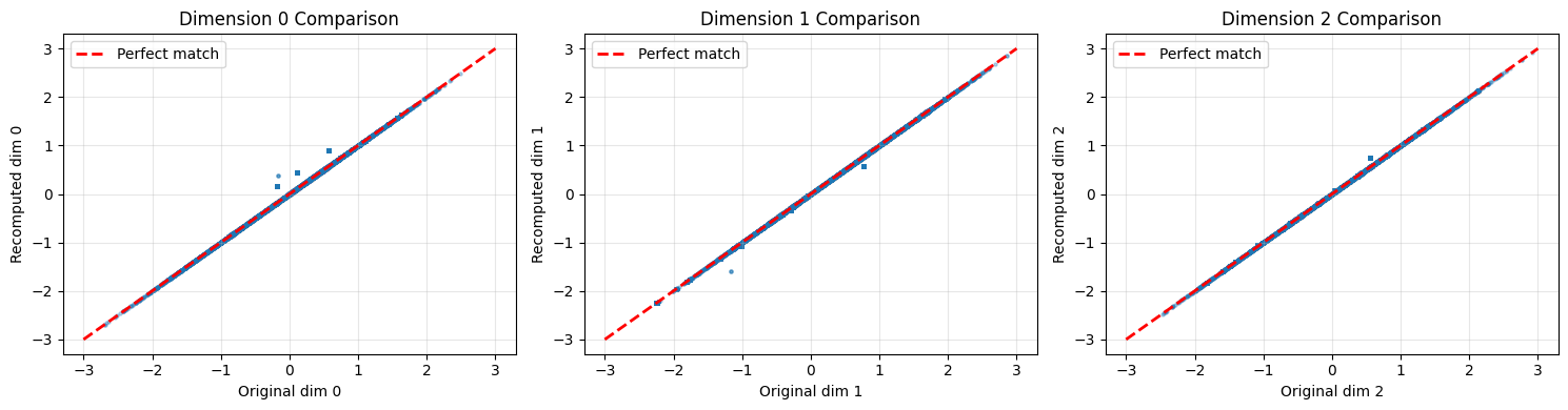
How to read these comparison charts
Each scatter plot compares one embedding dimension between the original (saved) and recomputed embeddings:
Points on the red dashed line: Perfect match between original and recomputed
Points clustered tightly around the line: Pipeline is working correctly
Scattered points: Something differs (device, precision, or code changes)
A small amount of scatter (differences < 0.0001) is acceptable due to floating-point precision differences between devices.
6. Process New Events
Demonstrate processing completely new OCSF events that weren’t in the training data.
Key consideration: New events may contain categorical values not seen during training. The pipeline handles this by mapping unknown values to the ‘UNKNOWN’ category.
# Create some synthetic new events
new_events = pd.DataFrame([
    {
        'time': 1704067200000,  # Jan 1, 2024 00:00:00
        'class_name': 'Web Resources Activity',
        'activity_name': 'Access',
        'status': 'Success',
        'level': 'informational',
        'service': 'api-gateway',
        'actor_user_name': 'new_user_123',  # Unknown user
        'http_request_method': 'GET',
        'http_request_url_path': '/api/v1/data',
        'severity_id': 1,
        'activity_id': 1,
        'status_id': 1,
        'duration': 150,
        'http_response_code': 200,
    },
    {
        'time': 1704070800000,  # Jan 1, 2024 01:00:00 (1 AM - suspicious)
        'class_name': 'Web Resources Activity',
        'activity_name': 'Create',
        'status': 'Success',
        'level': 'informational',
        'service': 'unknown-service',  # Unknown service
        'actor_user_name': 'admin',
        'http_request_method': 'POST',
        'http_request_url_path': '/admin/users',
        'severity_id': 2,
        'activity_id': 2,
        'status_id': 1,
        'duration': 500,
        'http_response_code': 201,
    },
    {
        'time': 1704153600000,  # Jan 2, 2024 00:00:00
        'class_name': 'Authentication',  # May be unknown class
        'activity_name': 'Logon',
        'status': 'Failure',
        'level': 'warning',
        'service': 'auth-service',
        'actor_user_name': 'unknown_user',
        'http_request_method': 'POST',
        'http_request_url_path': '/login',
        'severity_id': 3,
        'activity_id': 1,
        'status_id': 2,
        'duration': 50,
        'http_response_code': 401,
    }
])

print("New events to process:")
print(new_events[['time', 'activity_name', 'status', 'actor_user_name', 'http_response_code']])
New events to process:
time activity_name status actor_user_name http_response_code
0 1704067200000 Access Success new_user_123 200
1 1704070800000 Create Success admin 201
2 1704153600000 Logon Failure unknown_user 401
# Generate embeddings for new events
new_embeddings = pipeline.transform(new_events)

print(f"\nNew Event Embeddings:")
print(f"  Shape: {new_embeddings.shape}")
print(f"\nEmbedding statistics per event:")
for i, event in enumerate(['Normal API access', 'Suspicious 1AM admin', 'Failed auth']):
    emb = new_embeddings[i]
    print(f"  {event}:")
    print(f"    Mean: {emb.mean():.4f}, Std: {emb.std():.4f}, Norm: {np.linalg.norm(emb):.4f}")
New Event Embeddings:
  Shape: (3, 128)

Embedding statistics per event:
  Normal API access:
    Mean: 0.0038, Std: 1.0012, Norm: 11.3276
  Suspicious 1AM admin:
    Mean: 0.0040, Std: 0.9992, Norm: 11.3043
  Failed auth:
    Mean: 0.0040, Std: 1.0063, Norm: 11.3855
7. Find Similar Events
Use embeddings to find similar events in the training data.
What you should expect:
Similar events (same activity, status) should have high cosine similarity
Unusual events may have lower similarity to most training data
Cosine similarity ranges from -1 to 1 (higher = more similar)
from sklearn.metrics.pairwise import cosine_similarity

def find_similar_events(query_embedding, reference_embeddings, reference_df, top_k=5):
    """
    Find most similar events using cosine similarity.

    Returns indices and similarities of top-k matches.
    """
    # Compute similarities
    similarities = cosine_similarity([query_embedding], reference_embeddings)[0]

    # Get top-k indices
    top_indices = np.argsort(similarities)[::-1][:top_k]
    top_similarities = similarities[top_indices]

    return top_indices, top_similarities

# Find similar events for each new event
display_cols = ['activity_name', 'status', 'actor_user_name', 'http_response_code']
display_cols = [c for c in display_cols if c in df.columns]

print("Finding similar events in training data...\n")

for i, (name, emb) in enumerate(zip(
    ['Normal API access', 'Suspicious 1AM admin', 'Failed auth attempt'],
    new_embeddings
)):
    indices, sims = find_similar_events(emb, original_embeddings, df, top_k=3)

    print(f"=== {name} ===")
    print(f"Query: {new_events.iloc[i][display_cols].to_dict()}")
    print(f"\nTop 3 similar events (cosine similarity):")
    for idx, sim in zip(indices, sims):
        print(f"  Similarity: {sim:.4f}")
        print(f"    {df.iloc[idx][display_cols].to_dict()}")
    print()
Finding similar events in training data...
=== Normal API access ===
Query: {'activity_name': 'Access', 'status': 'Success', 'actor_user_name': 'new_user_123', 'http_response_code': 200}
Top 3 similar events (cosine similarity):
Similarity: 0.5926
{'activity_name': 'Unknown', 'status': 'Success', 'actor_user_name': None, 'http_response_code': nan}
Similarity: 0.5926
{'activity_name': 'Unknown', 'status': 'Success', 'actor_user_name': None, 'http_response_code': nan}
Similarity: 0.5926
{'activity_name': 'Unknown', 'status': 'Success', 'actor_user_name': None, 'http_response_code': nan}
=== Suspicious 1AM admin ===
Query: {'activity_name': 'Create', 'status': 'Success', 'actor_user_name': 'admin', 'http_response_code': 201}
Top 3 similar events (cosine similarity):
Similarity: 0.6274
{'activity_name': 'Create', 'status': 'Success', 'actor_user_name': 'carol.williams', 'http_response_code': 200.0}
Similarity: 0.6186
{'activity_name': 'Create', 'status': 'Success', 'actor_user_name': 'eve.davis', 'http_response_code': 200.0}
Similarity: 0.6116
{'activity_name': 'Create', 'status': 'Success', 'actor_user_name': 'carol.williams', 'http_response_code': 200.0}
=== Failed auth attempt ===
Query: {'activity_name': 'Logon', 'status': 'Failure', 'actor_user_name': 'unknown_user', 'http_response_code': 401}
Top 3 similar events (cosine similarity):
Similarity: 0.6675
{'activity_name': 'Unknown', 'status': 'Success', 'actor_user_name': None, 'http_response_code': nan}
Similarity: 0.6675
{'activity_name': 'Unknown', 'status': 'Success', 'actor_user_name': None, 'http_response_code': nan}
Similarity: 0.6675
{'activity_name': 'Unknown', 'status': 'Success', 'actor_user_name': None, 'http_response_code': nan}
8. Anomaly Scoring for New Events
Score new events against the training distribution.
What you should expect:
Normal events should have low anomaly scores (close to training data)
Unusual events (1 AM admin activity, failed auth) may have higher scores
Scores represent average distance to k-nearest training neighbors
from sklearn.neighbors import NearestNeighbors

# Fit k-NN on training embeddings
k = 20
knn = NearestNeighbors(n_neighbors=k, metric='cosine')
knn.fit(original_embeddings)

# Score new events
distances, _ = knn.kneighbors(new_embeddings)
anomaly_scores = distances.mean(axis=1)

# Compare to training distribution
train_distances, _ = knn.kneighbors(original_embeddings)
train_scores = train_distances[:, 1:].mean(axis=1)  # Exclude self

print("Anomaly Scores (k-NN distance):")
print(f"\nTraining data statistics:")
print(f"  Mean: {train_scores.mean():.4f}")
print(f"  Std: {train_scores.std():.4f}")
print(f"  95th percentile: {np.percentile(train_scores, 95):.4f}")

print(f"\nNew event scores:")
for name, score in zip(
    ['Normal API access', 'Suspicious 1AM admin', 'Failed auth attempt'],
    anomaly_scores
):
    percentile = (train_scores < score).mean() * 100
    flag = "⚠️ ANOMALY" if percentile > 95 else "✓ Normal"
    print(f"  {name}: {score:.4f} (percentile: {percentile:.1f}%) {flag}")
Anomaly Scores (k-NN distance):
Training data statistics:
Mean: 0.0694
Std: 0.1059
95th percentile: 0.2489
New event scores:
Normal API access: 0.4252 (percentile: 100.0%) ⚠️ ANOMALY
Suspicious 1AM admin: 0.4047 (percentile: 100.0%) ⚠️ ANOMALY
Failed auth attempt: 0.3631 (percentile: 100.0%) ⚠️ ANOMALY
# Visualize where new events fall in the score distribution
fig, ax = plt.subplots(figsize=(12, 5))

# Plot training distribution
ax.hist(train_scores, bins=50, alpha=0.7, label='Training data', color='blue', edgecolor='black')

# Mark 95th percentile threshold
threshold = np.percentile(train_scores, 95)
ax.axvline(threshold, color='red', linestyle='--', linewidth=2, label=f'95th percentile: {threshold:.4f}')

# Mark new events
colors = ['green', 'orange', 'red']
names = ['Normal API', 'Suspicious 1AM', 'Failed auth']
for score, color, name in zip(anomaly_scores, colors, names):
    ax.axvline(score, color=color, linewidth=3, label=f'{name}: {score:.4f}')

ax.set_xlabel('Anomaly Score (k-NN distance)')
ax.set_ylabel('Count')
ax.set_title('New Event Scores vs Training Distribution')
ax.legend(loc='upper right')
ax.grid(True, alpha=0.3)

plt.tight_layout()
plt.show()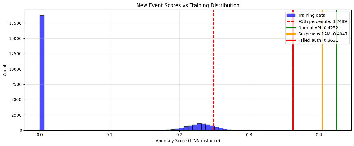
How to read this anomaly score chart
Blue histogram: Distribution of anomaly scores from training data (baseline)
Red dashed line: 95th percentile threshold - events beyond this are flagged as anomalies
Colored vertical lines: Where new events fall in the distribution
Interpretation:
Lines left of threshold (in the blue bulk): Normal events
Lines right of threshold (in the tail): Anomalous events
The further right, the more anomalous the event appears relative to training data
9. Save Pipeline for Production
Save everything needed for production inference.
Production deployment checklist:
Model weights (
tabular_resnet.pt)Feature artifacts (
feature_artifacts.pkl)Model class definition (copy to your codebase)
Training embeddings for anomaly scoring (optional)
# Save complete inference package
inference_package = {
    'model_state_dict': model.state_dict(),
    'model_config': {
        'num_numerical': len(numerical_cols),
        'cardinalities': cardinalities,
        'd_model': 128,
        'num_blocks': 4,
        'embedding_dim': 32,
        'dropout': 0.1
    },
    'feature_artifacts': artifacts,
    'training_stats': {
        'anomaly_score_mean': train_scores.mean(),
        'anomaly_score_std': train_scores.std(),
        'anomaly_score_95pct': float(np.percentile(train_scores, 95)),
        'training_samples': len(original_embeddings)
    }
}

torch.save(inference_package, '../data/inference_package.pt')
print("Saved complete inference package to ../data/inference_package.pt")
print("\nPackage contents:")
for key in inference_package:
    if isinstance(inference_package[key], dict):
        print(f"  {key}: {list(inference_package[key].keys())}")
    else:
        print(f"  {key}: {type(inference_package[key]).__name__}")
Saved complete inference package to ../data/inference_package.pt
Package contents:
model_state_dict: ['embeddings.0.weight', 'embeddings.1.weight', 'embeddings.2.weight', 'embeddings.3.weight', 'embeddings.4.weight', 'embeddings.5.weight', 'embeddings.6.weight', 'embeddings.7.weight', 'embeddings.8.weight', 'embeddings.9.weight', 'embeddings.10.weight', 'embeddings.11.weight', 'input_projection.weight', 'input_projection.bias', 'blocks.0.linear1.weight', 'blocks.0.linear1.bias', 'blocks.0.linear2.weight', 'blocks.0.linear2.bias', 'blocks.0.norm1.weight', 'blocks.0.norm1.bias', 'blocks.0.norm2.weight', 'blocks.0.norm2.bias', 'blocks.1.linear1.weight', 'blocks.1.linear1.bias', 'blocks.1.linear2.weight', 'blocks.1.linear2.bias', 'blocks.1.norm1.weight', 'blocks.1.norm1.bias', 'blocks.1.norm2.weight', 'blocks.1.norm2.bias', 'blocks.2.linear1.weight', 'blocks.2.linear1.bias', 'blocks.2.linear2.weight', 'blocks.2.linear2.bias', 'blocks.2.norm1.weight', 'blocks.2.norm1.bias', 'blocks.2.norm2.weight', 'blocks.2.norm2.bias', 'blocks.3.linear1.weight', 'blocks.3.linear1.bias', 'blocks.3.linear2.weight', 'blocks.3.linear2.bias', 'blocks.3.norm1.weight', 'blocks.3.norm1.bias', 'blocks.3.norm2.weight', 'blocks.3.norm2.bias', 'final_norm.weight', 'final_norm.bias']
model_config: ['num_numerical', 'cardinalities', 'd_model', 'num_blocks', 'embedding_dim', 'dropout']
feature_artifacts: ['encoders', 'scaler', 'categorical_cols', 'numerical_cols', 'cardinalities']
training_stats: ['anomaly_score_mean', 'anomaly_score_std', 'anomaly_score_95pct', 'training_samples']
10. Quick Reference: Loading in Production
Here’s a minimal example of using the saved model in production:
# Example: Load and use in production
def load_production_model(package_path, device='cpu'):
    """
    Load model from inference package.

    Usage:
        model, pipeline, stats = load_production_model('inference_package.pt')
        embeddings = pipeline.transform(new_events_df)
    """
    # Note: weights_only=False is required because the package contains sklearn
    # objects (LabelEncoder, StandardScaler). Only use this with trusted files.
    package = torch.load(package_path, map_location=device, weights_only=False)

    # Recreate model
    config = package['model_config']
    model = TabularResNet(
        num_numerical=config['num_numerical'],
        cardinalities=config['cardinalities'],
        d_model=config['d_model'],
        num_blocks=config['num_blocks'],
        embedding_dim=config['embedding_dim'],
        dropout=config['dropout']
    )
    model.load_state_dict(package['model_state_dict'])
    model = model.to(device)
    model.eval()

    # Create pipeline
    pipeline = OCSFEmbeddingPipeline(model, package['feature_artifacts'], device=device)

    return model, pipeline, package['training_stats']

# Demo
print("Loading production model...")
prod_model, prod_pipeline, stats = load_production_model('../data/inference_package.pt', device=device)

print(f"\nModel loaded. Training statistics:")
print(f"  Training samples: {stats['training_samples']}")
print(f"  Anomaly threshold (95%): {stats['anomaly_score_95pct']:.4f}")

# Quick test
test_emb = prod_pipeline.transform(new_events[:1])
print(f"\nTest inference successful. Embedding shape: {test_emb.shape}")
Loading production model...
Model loaded. Training statistics:
Training samples: 27084
Anomaly threshold (95%): 0.2489
Test inference successful. Embedding shape: (1, 128)
Summary
In this notebook, we:
Loaded trained model and feature artifacts
Built inference pipeline that handles the complete workflow
Verified reproducibility by comparing with saved embeddings
Processed new events including those with unknown categories
Found similar events using cosine similarity
Computed anomaly scores against training distribution
Saved production package with model, config, and statistics
Key takeaways:
Always save model config alongside weights
Include feature artifacts (encoders, scalers) for preprocessing
Handle unknown categorical values gracefully
Use training statistics for calibrating anomaly thresholds
Next: Use the model for anomaly detection on production data.