Learn how to train TabularResNet on unlabelled OCSF data using self-supervised learning techniques.
Note: Need OCSF data for training? See Appendix: Generating Training Data for a Docker Compose setup that generates ~72,000 realistic observability events with labeled anomalies.
What is Self-Supervised Learning?
The challenge: You have millions of OCSF observability logs but no labels telling you which are “normal” vs “anomalous”. Traditional supervised learning requires labeled data (e.g., “this event is anomalous”), which is expensive and often unavailable for new anomaly types.
The solution: Self-supervised learning creates training tasks automatically from the data itself, without human labels. The model learns useful representations by solving these artificial tasks.
Analogy: Think of it like learning a language by filling in blanks. If you read “The cat sat on the ___”, you can learn about cats and furniture even without explicit teaching. The sentence structure itself provides the supervision.
For tabular data, we use two main self-supervised approaches:
The Training Strategy
Since your observability data is unlabelled, you need self-supervised learning. Two effective approaches from the TabTransformer paper Huang et al. (2020):
Contrastive Learning - Recommended starting point: Train the model so similar records have similar embeddings. Simpler to implement, works with base TabularResNet (no model modifications needed)
Masked Feature Prediction (MFP) - Advanced technique: Hide features and train model to reconstruct them. Requires extending TabularResNet with prediction heads, more complex loss functions
Recommendation: Start with Contrastive Learning unless you have millions of records and want to invest time in hyperparameter tuning for MFP.
1. Contrastive Learning
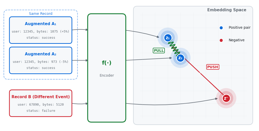
The idea: Train the model so that similar records have similar embeddings, while different records have different embeddings.
How it works:
For every record in your training data, create two augmented versions
Apply random noise: add ±5% to numerical features, randomly swap 10-20% of categorical values
Pass through encoder: Feed the augmented versions through the model (encoder
f(·)) to get embeddingsTrain the model so the two augmented versions have similar embeddings (they’re “positive pairs”)
Meanwhile, ensure embeddings from different original records stay far apart (they’re “negative pairs”)
Key point: We augment every single record in the batch, creating exactly 2 augmented copies per record. With a batch size of 256, we get 512 augmented samples (256 pairs).
Analogy: It’s like teaching someone to recognize faces. Show them two photos of the same person from different angles and say “these are the same.” Show them photos of different people and say “these are different.” Over time, they learn what makes faces similar or different.
Why this works: The model learns which variations in features are superficial (noise) vs meaningful (different events). Records with similar embeddings represent similar system behaviors, making it easy to detect anomalies as records with unusual embeddings.
Detailed augmentation process:
Q: Do we augment every data row? A: Yes, every single record in the batch is augmented.
There’s no selection process - we augment all samples.
Q: How many augmented copies per record? A: Exactly 2 copies per record (called views). These are created independently with different random noise.
Example: One OCSF login record → Augmented copy 1 (bytes +5%, user_id unchanged) + Augmented copy 2 (bytes -3%, user_id unchanged)
Q: What’s a typical batch size? A: 256-512 original records per batch, which gives you 512-1024 augmented samples.
With 256 original records → 512 augmented samples total
This creates 256 positive pairs (one pair per original record)
Each augmented sample contrasts against 510 negatives (all 512 samples except itself and its positive pair)
Total: each sample learns from 1 positive and 510 negatives
Q: Why create 2 copies and not 3 or 5? A: 2 copies is the standard because:
Creates one clear positive pair per original record
Computationally efficient (similarity matrix is 2N × 2N)
More copies would increase training time without proportional benefit
Q: How much augmentation noise should we apply? A: Light noise - enough to create variation but not so much that positive pairs appear unrelated:
Numerical features: ±5-15% Gaussian noise
Categorical features: 10-20% random swaps
Too little noise → model learns shortcuts (memorizes exact values)
Too much noise → positive pairs appear as negatives (model can’t learn)
Key terms:
Augmentation: Creating slightly modified versions of data (e.g., adding noise to numerical features)
Positive pairs: Two augmented versions of the same record (should have similar embeddings)
Negative pairs: Augmented versions from different records (should have different embeddings)
Temperature: A parameter controlling how strictly the model enforces similarity (lower = stricter)
SimCLR: A popular contrastive learning framework we adapt for tabular data
What we’re implementing: A complete SimCLR-style contrastive learning pipeline:
Augmentation class (
TabularAugmentation):Adds Gaussian noise to numerical features (e.g.,
bytes: 1024→bytes: 1038)Randomly swaps categorical values (e.g.,
status: success→status: failurewith 20% probability)Creates two independent augmented views of each record
Contrastive loss function (
contrastive_loss):Generates two augmented views per sample
Computes embeddings for all views
Normalizes embeddings (critical for cosine similarity)
Computes similarity matrix between all pairs
Applies softmax with temperature scaling
Uses cross-entropy loss to pull positive pairs together, push negatives apart
Implementation:
1 2 3 4 5 6 7 8 9 10 11 12 13 14 15 16 17 18 19 20 21 22 23 24 25 26 27 28 29 30 31 32 33 34 35 36 37 38 39 40 41 42 43 44 45 46 47 48 49 50 51 52 53 54 55 56 57 58 59 60 61 62 63 64 65 66 67 68 69 70 71 72 73 74 75 76 77 78 79 80 81 82 83 84 85 86 87 88 89 90 91 92 93import torch import torch.nn as nn import torch.nn.functional as F class TabularAugmentation: """ Data augmentation for tabular data used in contrastive learning. """ def __init__(self, noise_level=0.1, dropout_prob=0.2): self.noise_level = noise_level self.dropout_prob = dropout_prob def augment_numerical(self, numerical_features): """Add Gaussian noise to numerical features.""" noise = torch.randn_like(numerical_features) * self.noise_level return numerical_features + noise def augment_categorical(self, categorical_features, cardinalities): """Randomly replace some categorical features with random values.""" augmented = categorical_features.clone() mask = torch.rand_like(categorical_features.float()) < self.dropout_prob for i, cardinality in enumerate(cardinalities): # Replace masked values with random categories random_cats = torch.randint(0, cardinality, (categorical_features.size(0),), device=categorical_features.device) augmented[:, i] = torch.where(mask[:, i], random_cats, categorical_features[:, i]) return augmented def contrastive_loss(model, numerical, categorical, cardinalities, temperature=0.07, augmenter=None): """ SimCLR-style contrastive loss for tabular data. Args: model: TabularResNet model numerical: (batch_size, num_numerical) numerical features categorical: (batch_size, num_categorical) categorical features cardinalities: List of cardinalities for categorical features temperature: Temperature parameter for softmax augmenter: TabularAugmentation instance Returns: Contrastive loss value """ if augmenter is None: augmenter = TabularAugmentation() batch_size = numerical.size(0) # Create two augmented views of each sample # View 1: First augmentation num_aug1 = augmenter.augment_numerical(numerical) cat_aug1 = augmenter.augment_categorical(categorical, cardinalities) embeddings1 = model(num_aug1, cat_aug1, return_embedding=True) # View 2: Second augmentation (independent) num_aug2 = augmenter.augment_numerical(numerical) cat_aug2 = augmenter.augment_categorical(categorical, cardinalities) embeddings2 = model(num_aug2, cat_aug2, return_embedding=True) # Concatenate both views: [emb1_batch, emb2_batch] embeddings = torch.cat([embeddings1, embeddings2], dim=0) # Normalize embeddings (important for cosine similarity) embeddings = F.normalize(embeddings, dim=1) # Compute similarity matrix: (2*batch_size, 2*batch_size) similarity_matrix = torch.matmul(embeddings, embeddings.T) / temperature # Create labels: positive pairs are (i, i+batch_size) and (i+batch_size, i) # For sample i: positive is at index i+batch_size labels = torch.cat([ torch.arange(batch_size, 2 * batch_size), # For first half torch.arange(0, batch_size) # For second half ], dim=0).to(numerical.device) # Mask to remove self-similarity (diagonal) mask = torch.eye(2 * batch_size, dtype=torch.bool, device=numerical.device) similarity_matrix = similarity_matrix.masked_fill(mask, float('-inf')) # Compute cross-entropy loss # Each row: softmax over all other samples, target is the positive pair loss = F.cross_entropy(similarity_matrix, labels) return loss # Example usage (needs TabularResNet from Part 2) print("Contrastive learning setup complete") print("Use contrastive_loss() with your TabularResNet model for self-supervised training")
How the contrastive loss works step-by-step:
Augmentation (lines 56-63):
Original batch of 64 records → augment twice → 2 views of 64 records each
Each view sees slightly different data (noise + dropout)
Embedding (lines 58, 63):
Pass both views through TabularResNet → get embeddings
Each embedding is a dense vector (e.g., 256-dimensional)
Normalization (line 69):
Normalize embeddings to unit vectors:
embedding / ||embedding||Critical for using cosine similarity (PyTorch F.normalize docs)
Similarity matrix (line 72):
Compute dot product between all pairs:
embeddings @ embeddings.TResults in (128, 128) matrix where entry (i,j) = similarity between sample i and j
Divide by temperature (0.07) to scale similarities (SimCLR paper for temperature explanation)
Positive pair labels (lines 76-79):
For sample i in first view, its positive pair is sample i in second view (index i + batch_size)
For sample i in second view, its positive pair is sample i in first view (index i - batch_size)
Cross-entropy loss (line 87):
Treat as classification: for each sample, predict which of the 127 other samples is its positive pair
Loss pulls positive pairs together, pushes negatives apart
Hyperparameter tuning:
noise_level (default 0.1): Controls augmentation strength for numerical features
Too low (0.01) → views too similar, model learns shortcuts (e.g., memorizes noise patterns)
Too high (0.5) → views too different, positive pairs appear as negatives
Start with 0.1 and adjust based on validation performance
dropout_prob (default 0.2): Probability of swapping categorical values
Higher values create more diverse augmentations but risk semantic changes
For observability logs, keep low (0.1-0.2) to avoid changing event meaning
temperature (default 0.07): Controls similarity scaling
Lower (0.01) → sharper gradients, model focuses on hardest negatives
Higher (0.5) → softer gradients, model considers all negatives equally
SimCLR paper found 0.07 works best empirically
Pitfalls:
Batch size matters: Contrastive learning needs large batches (256-1024) to provide enough negative samples. Small batches (32) don’t work well - model has too few negatives to learn from
GPU memory: Large batches require lots of memory. If OOM, use gradient accumulation or reduce model size
Augmentation quality: Bad augmentations break contrastive learning by creating false positive pairs. For OCSF observability data, this is critical:
Why this matters: The model learns that “these two augmented views are the same event.” If augmentation changes the semantic meaning, you’re teaching the model that fundamentally different events are similar.
What NOT to augment:
❌ Operational outcomes: Don’t swap
status: success↔status: failure(completely different event types)❌ Event types: Don’t change
activity_idorclass_uid(these define what happened)❌ Critical identifiers: Be careful with
user_id,src_endpoint.ip,dst_endpoint.ip(swapping creates wrong associations)❌ Severity levels: Don’t change
severityorrisk_level(changes event importance)
What to augment safely:
✅ Numerical metrics: Add small noise to
bytes,duration,count(±5-15%)✅ Timestamps: Slight time jitter (±few seconds) for
time,end_time✅ Non-critical categorical: Randomly mask
http_request.user_agent,file.name(with domain-appropriate values)✅ Metadata: Change
observables.type_id,unmappedfields that don’t affect operational meaning
Example of good vs bad augmentation:
# Original OCSF login event
original = {
    'activity_id': 1,  # Logon
    'status': 'success',
    'user_id': 12345,
    'bytes': 1024,
    'duration': 5.2
}

# ✅ GOOD: Preserves semantic meaning
good_augment = {
    'activity_id': 1,  # Same - logon
    'status': 'success',  # Same - successful
    'user_id': 12345,  # Same user
    'bytes': 1075,  # +5% noise
    'duration': 5.4   # +4% noise
}

# ❌ BAD: Changes semantic meaning
bad_augment = {
    'activity_id': 2,  # WRONG - changed to Logoff!
    'status': 'failure',  # WRONG - now a failed event!
    'user_id': 67890,  # WRONG - different user!
    'bytes': 1075,
    'duration': 5.4
}
How to detect bad augmentation: If your model learns that successful logins and failed logins have similar embeddings, or that different users appear similar, your augmentation is too aggressive. Check embedding clusters (Part 5) to verify meaningful events separate properly.
Computational cost: Computing similarity matrix is O(batch_size²). With batch_size=1024, that’s 1M similarity computations per step
Further reading:
SimCLR paper - Original contrastive learning framework
PyTorch contrastive learning tutorial - General training patterns
Temperature in contrastive learning - Deep dive on temperature parameter
2. Masked Feature Prediction (MFP) [DRAFT]
The idea: Hide some features in your data and train the model to predict what’s missing.
How it works:
Take an OCSF record:
{user_id: 12345, status: success, bytes: 1024, duration: 5.2}Randomly mask 15% of features:
{user_id: [MASK], status: success, bytes: 1024, duration: [MASK]}Train the model to predict the masked values:
user_id = 12345,duration = 5.2
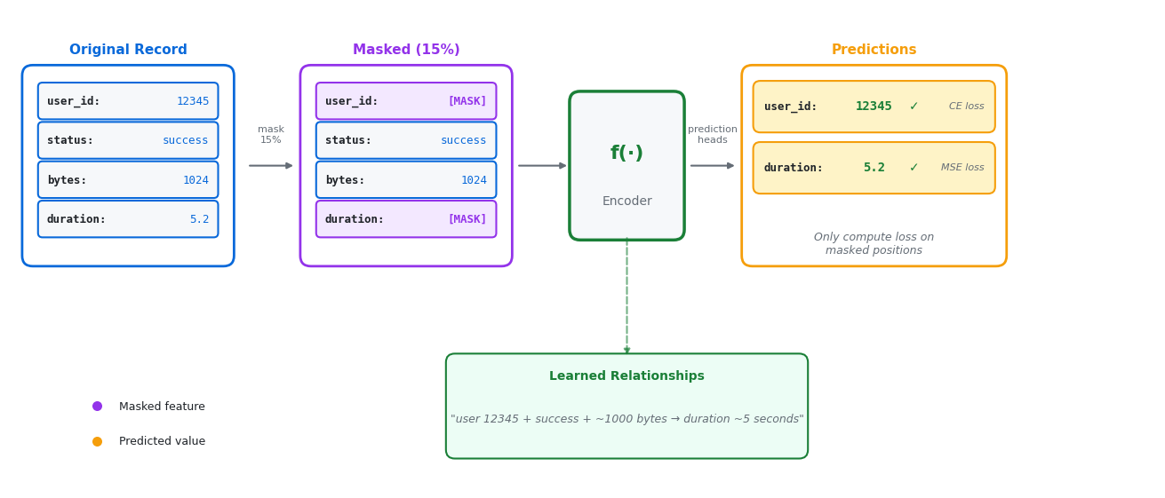
Why this works: To predict missing features, the model must learn relationships between features (e.g., “successful logins from user 12345 typically transfer ~1000 bytes in ~5 seconds”). These learned relationships create useful embeddings that capture “normal” behavior patterns.
Key term:
Prediction heads: Additional linear layers added on top of the encoder that project embeddings back to the original feature space. For MFP, you need one head per categorical feature (outputs logits over possible values) and one head for all numerical features (outputs continuous predictions).
What MFP requires:
Model extension: Add prediction heads to TabularResNet (linear layers that project embeddings → original feature space)
Masking logic: Randomly hide 15% of features (both categorical and numerical)
Loss computation: Cross-entropy for categoricals, MSE for numericals, computed only on masked positions
Note: The base TabularResNet from Part 2 doesn’t include prediction heads. The complete implementation below shows how to extend it with categorical_predictors (ModuleList of linear layers, one per categorical feature) and numerical_predictor (single linear layer for all numerical features).
Complete MFP Implementation
Adding prediction heads to TabularResNet:
1 2 3 4 5 6 7 8 9 10 11 12 13 14 15 16 17 18 19 20 21 22 23 24 25 26 27 28 29 30 31 32 33 34 35 36 37 38 39 40 41 42 43 44 45 46 47 48 49 50 51 52 53 54 55 56 57 58 59 60import torch.nn as nn class TabularResNetWithMFP(nn.Module): """ TabularResNet extended with Masked Feature Prediction heads. Adds linear layers to project embeddings back to feature space for reconstructing masked values. """ def __init__(self, base_model, categorical_cardinalities, num_numerical): super().__init__() self.base_model = base_model # Original TabularResNet self.d_model = base_model.d_model # Prediction heads for categorical features # One linear layer per categorical feature self.categorical_predictors = nn.ModuleList([ nn.Linear(self.d_model, cardinality) for cardinality in categorical_cardinalities ]) # Prediction head for numerical features # Single linear layer outputting all numerical features self.numerical_predictor = nn.Linear(self.d_model, num_numerical) def forward(self, numerical, categorical, return_embedding=False): # Get embedding from base model embedding = self.base_model(numerical, categorical, return_embedding=True) if return_embedding: return embedding # Predict categorical features (for MFP training) cat_predictions = [pred(embedding) for pred in self.categorical_predictors] cat_predictions = torch.stack(cat_predictions, dim=1) # (batch, num_cat, vocab_size) # Predict numerical features (for MFP training) num_predictions = self.numerical_predictor(embedding) # (batch, num_numerical) return cat_predictions, num_predictions # Usage example from part2 import TabularResNet # Import from Part 2 # Create base model base_model = TabularResNet( num_numerical_features=50, categorical_cardinalities=[100, 50, 200, 1000], d_model=256, num_blocks=6 ) # Extend with MFP heads model_with_mfp = TabularResNetWithMFP( base_model=base_model, categorical_cardinalities=[100, 50, 200, 1000], num_numerical=50 ) print("Extended model ready for MFP training")
Understanding the prediction heads:
categorical_predictors(lines 17-20): AModuleListcontaining one linear layer per categorical featureIf you have 4 categorical features with cardinalities [100, 50, 200, 1000], you get 4 linear layers:
Layer 0:
Linear(d_model=256, output=100)- predicts values for categorical feature 0 (100 possible values)Layer 1:
Linear(d_model=256, output=50)- predicts values for categorical feature 1 (50 possible values)Layer 2:
Linear(d_model=256, output=200)- predicts values for categorical feature 2Layer 3:
Linear(d_model=256, output=1000)- predicts values for categorical feature 3
Each layer takes the embedding (256-dim) and outputs logits for that feature’s vocabulary
Line 34: Uses list comprehension to apply each predictor to the embedding
Line 35: Stacks predictions into a single tensor of shape
(batch, num_categorical, vocab_size)
numerical_predictor(line 24): A single linear layer for all numerical featuresIf you have 50 numerical features:
Linear(d_model=256, output=50)Takes embedding (256-dim) and outputs predictions for all 50 numerical values at once
Line 38: Single forward pass predicts all numerical features simultaneously
Uses MSE loss (continuous values), not cross-entropy
Complete MFP loss with both categorical and numerical masking:
def complete_masked_feature_prediction_loss(model, numerical, categorical,
                                           mask_prob=0.15):
    """
    Complete MFP loss masking both categorical and numerical features.

    Args:
        model: TabularResNetWithMFP instance
        numerical: (batch_size, num_numerical) tensor
        categorical: (batch_size, num_categorical) tensor
        mask_prob: Probability of masking each feature

    Returns:
        Combined loss for categorical and numerical predictions
    """
    batch_size = numerical.size(0)

    # --- Mask categorical features ---
    masked_categorical = categorical.clone()
    cat_mask = torch.rand_like(categorical.float()) < mask_prob
    masked_categorical[cat_mask] = 0  # 0 = [MASK] token

    # --- Mask numerical features ---
    masked_numerical = numerical.clone()
    num_mask = torch.rand_like(numerical) < mask_prob
    masked_numerical[num_mask] = 0  # Replace with 0 (could also use mean)

    # --- Get predictions ---
    cat_predictions, num_predictions = model(masked_numerical, masked_categorical)

    # --- Categorical loss (cross-entropy) ---
    # cat_predictions: (batch, num_categorical, vocab_size)
    # Need to reshape for cross_entropy
    cat_loss = 0
    num_cat_masked = 0

    for i in range(categorical.size(1)):  # For each categorical feature
        mask_i = cat_mask[:, i]
        if mask_i.sum() > 0:  # If any values masked
            pred_i = cat_predictions[:, i, :]  # (batch, vocab_size)
            target_i = categorical[:, i]  # (batch,)
            # Compute loss only on masked positions
            loss_i = F.cross_entropy(pred_i[mask_i], target_i[mask_i])
            cat_loss += loss_i
            num_cat_masked += 1

    cat_loss = cat_loss / max(num_cat_masked, 1)  # Average over features

    # --- Numerical loss (MSE) ---
    num_loss = F.mse_loss(
        num_predictions[num_mask],
        numerical[num_mask]
    )

    # --- Combined loss ---
    total_loss = cat_loss + num_loss

    return total_loss

# Usage in training loop
optimizer = torch.optim.Adam(model_with_mfp.parameters(), lr=1e-4)

for epoch in range(num_epochs):
    for numerical, categorical in dataloader:
        loss = complete_masked_feature_prediction_loss(
            model_with_mfp, numerical, categorical
        )

        optimizer.zero_grad()
        loss.backward()
        optimizer.step()
Why MFP is more complex than contrastive learning:
Requires model modification: Must add prediction heads (additional parameters to train)
Feature-specific losses: Different loss functions for categorical (cross-entropy) vs numerical (MSE)
Masking strategy: Need to decide how to mask (0, mean, learned token)
Computational overhead: Forward pass through prediction heads for every batch
Recommendation: For most users, start with Contrastive Learning which:
Works with base TabularResNet (no modifications needed)
Single loss function (contrastive loss)
Proven to work well for tabular data
Simpler implementation and debugging
Only add MFP if:
You have very large datasets (millions of records) where MFP’s explicit feature learning helps
You want to combine both approaches (MFP + contrastive) for maximum performance
You’re willing to invest time in hyperparameter tuning (mask probability, loss weighting)
Additional MFP pitfalls:
Masking strategy tuning: 15% mask probability works for BERT but may need adjustment for tabular data. Try 10-20% range
Loss balancing: When combining categorical + numerical losses, you may need to weight them (e.g.,
total_loss = cat_loss + 0.5 * num_loss)Prediction head capacity: If prediction heads are too small, they bottleneck learning. Use
d_modellarge enough to capture feature complexityCold start: Model performs poorly in early epochs as it learns to reconstruct. Be patient or initialize with contrastive pre-training
Complete Training Loop
Now let’s put it all together. The code below shows a complete training pipeline including:
Dataset creation from OCSF numerical and categorical features
Training function that runs contrastive learning for multiple epochs
Example usage with simulated OCSF data
Why this code matters: This is the actual training loop you’ll use in production. Understanding the data flow (Dataset → DataLoader → Model → Loss → Optimizer) is crucial for customizing the training process to your specific OCSF schema.
import torch
from torch.utils.data import Dataset, DataLoader

class OCSFDataset(Dataset):
    """
    Dataset for OCSF observability data.
    """
    def __init__(self, numerical_data, categorical_data):
        """
        Args:
            numerical_data: (num_samples, num_numerical_features) numpy array
            categorical_data: (num_samples, num_categorical_features) numpy array
        """
        self.numerical = torch.FloatTensor(numerical_data)
        self.categorical = torch.LongTensor(categorical_data)

    def __len__(self):
        return len(self.numerical)

    def __getitem__(self, idx):
        return self.numerical[idx], self.categorical[idx]

def train_self_supervised(model, dataloader, optimizer, cardinalities,
                         num_epochs=50, device='cpu'):
    """
    Train TabularResNet using contrastive learning.

    Args:
        model: TabularResNet model
        dataloader: DataLoader with (numerical, categorical) batches
        optimizer: PyTorch optimizer
        cardinalities: List of categorical feature cardinalities
        num_epochs: Number of training epochs
        device: 'cuda' or 'cpu'

    Returns:
        List of loss values per epoch
    """
    model = model.to(device)
    model.train()

    augmenter = TabularAugmentation(noise_level=0.1, dropout_prob=0.2)
    losses = []

    for epoch in range(num_epochs):
        epoch_loss = 0.0
        num_batches = 0

        for numerical, categorical in dataloader:
            numerical = numerical.to(device)
            categorical = categorical.to(device)

            # Compute contrastive loss
            loss = contrastive_loss(model, numerical, categorical,
                                   cardinalities, augmenter=augmenter)

            # Backpropagation
            optimizer.zero_grad()
            loss.backward()
            optimizer.step()

            epoch_loss += loss.item()
            num_batches += 1

        avg_loss = epoch_loss / num_batches
        losses.append(avg_loss)

        if (epoch + 1) % 10 == 0:
            print(f"Epoch {epoch+1}/{num_epochs}: Loss = {avg_loss:.4f}")

    return losses

# Example usage (with dummy data)
import numpy as np

# Simulate OCSF data
num_samples = 10000
num_numerical = 50
num_categorical = 4
categorical_cardinalities = [100, 50, 200, 1000]

# Create dummy dataset
np.random.seed(42)
numerical_data = np.random.randn(num_samples, num_numerical)
categorical_data = np.random.randint(0, 50, (num_samples, num_categorical))

# Create dataset and dataloader
dataset = OCSFDataset(numerical_data, categorical_data)
dataloader = DataLoader(dataset, batch_size=256, shuffle=True, num_workers=0)

print(f"Dataset created: {len(dataset)} samples")
print(f"Numerical features: {num_numerical}")
print(f"Categorical features: {num_categorical}")
print(f"Ready for self-supervised training")
Dataset created: 10000 samples
Numerical features: 50
Categorical features: 4
Ready for self-supervised training
What this training loop does:
OCSFDataset class (lines 291-308):
Wraps numerical and categorical arrays as a PyTorch Dataset
Converts numpy arrays to tensors (FloatTensor for numerical, LongTensor for categorical)
Enables batch loading with DataLoader
train_self_supervised function (lines 310-358):
Main training loop that runs for
num_epochsiterationsEach epoch: iterate through all batches, compute loss, backpropagate, update weights
Uses optimizer
.zero _grad() to clear gradients before each step Uses loss.backward() to compute gradients
Uses optimizer.step() to update model weights
Example usage (lines 360-382):
Creates dummy data matching OCSF structure (50 numerical features, 4 categorical)
Wraps in Dataset and DataLoader with batch_size=256
Ready to call
train_self_supervised(model, dataloader, optimizer, ...)
What to monitor during training:
Loss curve: Should decrease steadily. If it plateaus after 10 epochs, try:
Increase learning rate (from 1e-4 to 1e-3)
Increase batch size (from 256 to 512)
Add more augmentation (increase noise_level from 0.1 to 0.15)
GPU utilization: Should be >80% during training. Low utilization means:
Batch size too small → increase batch size
Data loading bottleneck → increase
num_workersin DataLoaderCPU preprocessing slow → preprocess data once before training
Memory usage: If you hit OOM (out of memory):
Reduce batch_size (from 512 to 256)
Reduce d_model (from 512 to 256)
Reduce num_blocks (from 8 to 6)
Use mixed precision training (torch.cuda.amp)
Typical training time:
10K OCSF events: ~5 minutes on CPU, ~1 minute on GPU
1M events: ~2 hours on GPU (batch_size=512, num_epochs=50)
10M events: ~20 hours on GPU or use distributed training
Pitfalls:
No validation set: The example trains on all data without a validation split. For production, split 80/20 train/val and monitor validation loss to detect overfitting
Fixed epochs: Training for exactly 50 epochs may under/overfit. Use early stopping: stop when validation loss stops decreasing for 5 epochs
No checkpointing: If training crashes at epoch 45, you lose everything. Save model checkpoint every 10 epochs using torch.save()
Hardcoded device: Code assumes CPU. For GPU training, change
device='cuda'and ensure data is on same device
Production training script (recommended additions):
# Early stopping
best_val_loss = float('inf')
patience = 5
patience_counter = 0

for epoch in range(num_epochs):
    # ... training code ...

    # Validate
    val_loss = validate(model, val_dataloader)

    # Early stopping
    if val_loss < best_val_loss:
        best_val_loss = val_loss
        patience_counter = 0
        torch.save(model.state_dict(), 'best_model.pth')
    else:
        patience_counter += 1
        if patience_counter >= patience:
            print(f"Early stopping at epoch {epoch}")
            break
Training Best Practices
Note on Data Types: While the examples use OCSF observability logs, self-supervised learning works identically for any structured observability data (telemetry, traces, configs, application logs). The training pipeline (Dataset → DataLoader → Model → Loss) remains the same—just change the feature columns to match your data schema.
1. Data Preprocessing
Before training, you need to prepare your data (OCSF logs, metrics, traces, etc.). This involves:
StandardScaler: Normalizes numerical features to have mean=0 and std=1 (prevents features with large values from dominating)
LabelEncoder: Converts categorical strings to integers (e.g.,
"login" → 0,"logout" → 1)
from sklearn.preprocessing import StandardScaler, LabelEncoder

def preprocess_ocsf_data(df, numerical_cols, categorical_cols):
    """
    Preprocess OCSF DataFrame for training.

    Args:
        df: Pandas DataFrame with OCSF data
        numerical_cols: List of numerical column names
        categorical_cols: List of categorical column names

    Returns:
        (numerical_array, categorical_array, encoders, scaler)
    """
    # Standardize numerical features
    scaler = StandardScaler()
    numerical_data = scaler.fit_transform(df[numerical_cols].fillna(0))

    # Encode categorical features
    encoders = {}
    categorical_data = []

    for col in categorical_cols:
        encoder = LabelEncoder()
        # Handle unseen categories by adding an "unknown" category
        encoded = encoder.fit_transform(df[col].fillna('MISSING').astype(str))
        categorical_data.append(encoded)
        encoders[col] = encoder

    categorical_data = np.column_stack(categorical_data)

    return numerical_data, categorical_data, encoders, scaler
2. Hyperparameter Tuning
Hyperparameters control how your model learns and generalize. Getting them right can mean the difference between embeddings that clearly separate anomalies and embeddings that don’t work at all.
Key hyperparameters to tune:
| Parameter | Default | Range | Impact |
|---|---|---|---|
d_model | 256 | 128-512 | Embedding capacity |
num_blocks | 6 | 4-12 | Model depth |
dropout | 0.1 | 0.0-0.3 | Regularization |
batch_size | 256 | 64-512 | Training stability |
learning_rate | 1e-3 | 1e-4 to 1e-2 | Convergence speed |
temperature | 0.07 | 0.05-0.2 | Contrastive learning difficulty |
Recommendation: Start with defaults, then tune learning rate and batch size first.
3. Learning Rate Scheduling
from torch.optim.lr_scheduler import CosineAnnealingLR

# Example training with LR scheduling
optimizer = torch.optim.AdamW(model.parameters(), lr=1e-3, weight_decay=1e-4)
scheduler = CosineAnnealingLR(optimizer, T_max=num_epochs, eta_min=1e-5)

for epoch in range(num_epochs):
    # Training loop
    train_loss = train_epoch(...)

    # Step the scheduler
    scheduler.step()

    print(f"Epoch {epoch}: Loss={train_loss:.4f}, LR={scheduler.get_last_lr()[0]:.6f}")
4. Early Stopping
class EarlyStopping:
    """
    Early stopping to prevent overfitting.
    """
    def __init__(self, patience=10, min_delta=1e-4):
        self.patience = patience
        self.min_delta = min_delta
        self.counter = 0
        self.best_loss = None
        self.early_stop = False

    def __call__(self, val_loss):
        if self.best_loss is None:
            self.best_loss = val_loss
        elif val_loss > self.best_loss - self.min_delta:
            self.counter += 1
            if self.counter >= self.patience:
                self.early_stop = True
        else:
            self.best_loss = val_loss
            self.counter = 0

        return self.early_stop

# Usage
early_stopping = EarlyStopping(patience=10)

for epoch in range(num_epochs):
    train_loss = train_epoch(...)
    val_loss = validate(...)

    if early_stopping(val_loss):
        print(f"Early stopping at epoch {epoch}")
        break
Practical Workflow for OCSF Data
Step-by-Step Training Pipeline
def train_ocsf_anomaly_detector(
    ocsf_df,
    numerical_cols,
    categorical_cols,
    d_model=256,
    num_blocks=6,
    num_epochs=100,
    batch_size=256,
    device='cuda'
):
    """
    Complete pipeline to train custom TabularResNet embedding model on OCSF data.

    Args:
        ocsf_df: DataFrame with OCSF records
        numerical_cols: List of numerical column names
        categorical_cols: List of categorical column names
        d_model: Model hidden dimension
        num_blocks: Number of residual blocks
        num_epochs: Training epochs
        batch_size: Batch size
        device: 'cuda' or 'cpu'

    Returns:
        Trained model, scaler, and encoders
    """
    # 1. Preprocess data
    print("Preprocessing data...")
    numerical_data, categorical_data, encoders, scaler = preprocess_ocsf_data(
        ocsf_df, numerical_cols, categorical_cols
    )

    # 2. Create dataset and dataloader
    print("Creating dataset...")
    dataset = OCSFDataset(numerical_data, categorical_data)
    dataloader = DataLoader(dataset, batch_size=batch_size, shuffle=True, num_workers=4)

    # 3. Initialize model
    print("Initializing model...")
    categorical_cardinalities = [
        len(encoders[col].classes_) for col in categorical_cols
    ]

    # Import TabularResNet from Part 2
    from part2_tabular_resnet import TabularResNet

    model = TabularResNet(
        num_numerical_features=len(numerical_cols),
        categorical_cardinalities=categorical_cardinalities,
        d_model=d_model,
        num_blocks=num_blocks,
        dropout=0.1,
        num_classes=None  # Embedding mode
    )

    # 4. Setup optimizer
    optimizer = torch.optim.AdamW(model.parameters(), lr=1e-3, weight_decay=1e-4)
    scheduler = CosineAnnealingLR(optimizer, T_max=num_epochs)

    # 5. Train
    print(f"Training for {num_epochs} epochs...")
    losses = train_self_supervised(
        model, dataloader, optimizer, categorical_cardinalities,
        num_epochs=num_epochs, device=device
    )

    # 6. Save model
    checkpoint = {
        'model_state_dict': model.state_dict(),
        'scaler': scaler,
        'encoders': encoders,
        'categorical_cols': categorical_cols,
        'numerical_cols': numerical_cols,
        'hyperparameters': {
            'd_model': d_model,
            'num_blocks': num_blocks,
            'categorical_cardinalities': categorical_cardinalities
        }
    }

    torch.save(checkpoint, 'ocsf_anomaly_detector.pt')
    print("Model saved to ocsf_anomaly_detector.pt")

    return model, scaler, encoders

# Example usage (uncomment to run)
# model, scaler, encoders = train_ocsf_anomaly_detector(
#     ocsf_df=my_dataframe,
#     numerical_cols=['network_bytes_in', 'duration', ...],
#     categorical_cols=['user_id', 'status_id', 'entity_id', ...],
#     num_epochs=50
# )
Summary
In this part, you learned:
Two self-supervised approaches: Contrastive Learning (recommended starting point) and Masked Feature Prediction
Contrastive learning implementation with TabularAugmentation
Complete training loop with best practices
Hyperparameter tuning strategies
End-to-end pipeline for OCSF data
Next: In Part 5, we’ll learn how to evaluate the quality of learned embeddings using visualization and quantitative metrics.
References
- Huang, X., Khetan, A., Cvitkovic, M., & Karnin, Z. (2020). TabTransformer: Tabular Data Modeling Using Contextual Embeddings. arXiv Preprint arXiv:2012.06678.